Sparse generalized linear model (GLM)

A demonstration of sparse GLM regression using SparseReg toolbox. Sparsity is in the general sense: variable selection, total variation regularization, polynomial trend filtering, and others. Various penalties are implemented: elestic net (enet), power family (bridge regression), log penalty, SCAD, and MCP.

Sparse logistic regression (n>p)
Fused logistic regression
Sparse logistic regression (n<p)
Sparse loglinear (Poisson) regression (n>p)
Fused loglinear (Poisson) regression
Sparse loglinear (Poisson) regression (n<<p)

Sparse logistic regression (n>p)

Simulate a sample data set (n=500, p=50)

clear;
n = 500;
p = 50;

X = randn(n,p);             % generate a random design matrix
X = bsxfun(@rdivide, X, sqrt(sum(X.^2,1))); % normalize predictors
X = [ones(size(X,1),1) X];
b = zeros(p+1,1);           % true signalfirst ten predictors are 5
b(2:6) = 1;                 % first 5 predictors are 1
b(7:11) = -1;               % next 5 predictors are -1
inner = X*b;                % linear parts
prob = 1./(1+exp(-inner));
y = double(rand(n,1)<prob);

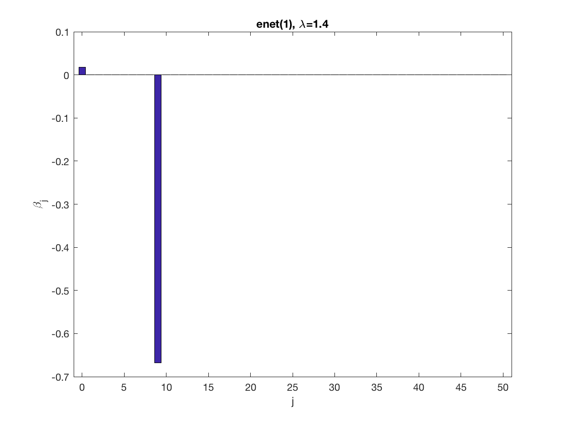
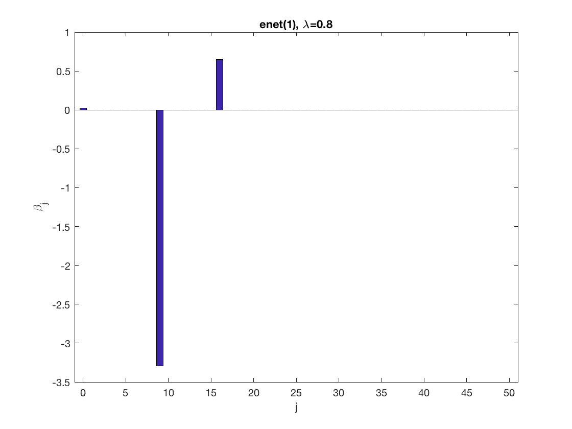
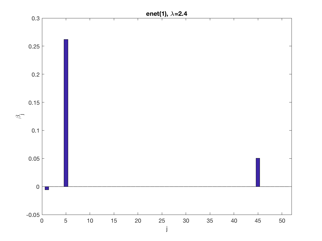
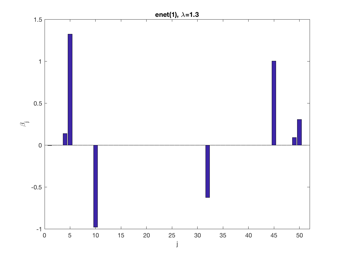
Sparse logistic regression at a fixed tuning parameter value

model = 'logistic';         % set model to logistic
penidx = [false; true(size(X,2)-1,1)];  % leave intercept unpenalized
penalty = 'enet';           % set penalty to lasso
penparam = 1;
lambdastart = 0;            % find the maximum tuning parameter to start
for j=1:size(X,2)
    if (penidx(j))
    lambdastart = max(lambdastart, ...
        glm_maxlambda(X(:,j),y,model,'penalty',penalty,'penparam',penparam));
    end
end
disp(lambdastart);

lambda = 0.9*lambdastart;   % tuning parameter value
betahat = ...               % sparse regression
    glm_sparsereg(X,y,lambda,model,'penidx',penidx,'penalty',penalty,...
    'penparam',penparam);

figure;                     % plot penalized estimate
bar(0:length(betahat)-1,betahat);
xlabel('j');
ylabel('\beta_j');
xlim([-1,length(betahat)]);
title([penalty '(' num2str(penparam) '), \lambda=' num2str(lambda,2)]);

lambda = 0.5*lambdastart;   % tuning parameter value
betahat = ...               % sparse regression
    glm_sparsereg(X,y,lambda,model,'penidx',penidx,'penalty',penalty,...
    'penparam',penparam);

figure;                     % plot penalized estimate
bar(0:length(betahat)-1,betahat);
xlabel('j');
ylabel('\beta_j');
xlim([-1,length(betahat)]);
title([penalty '(' num2str(penparam) '), \lambda=' num2str(lambda,2)]);

    1.6094

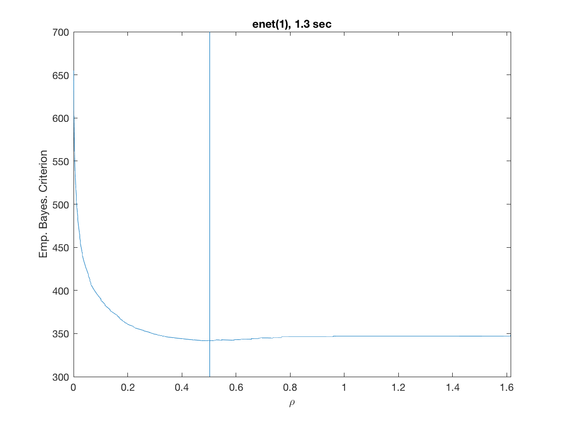
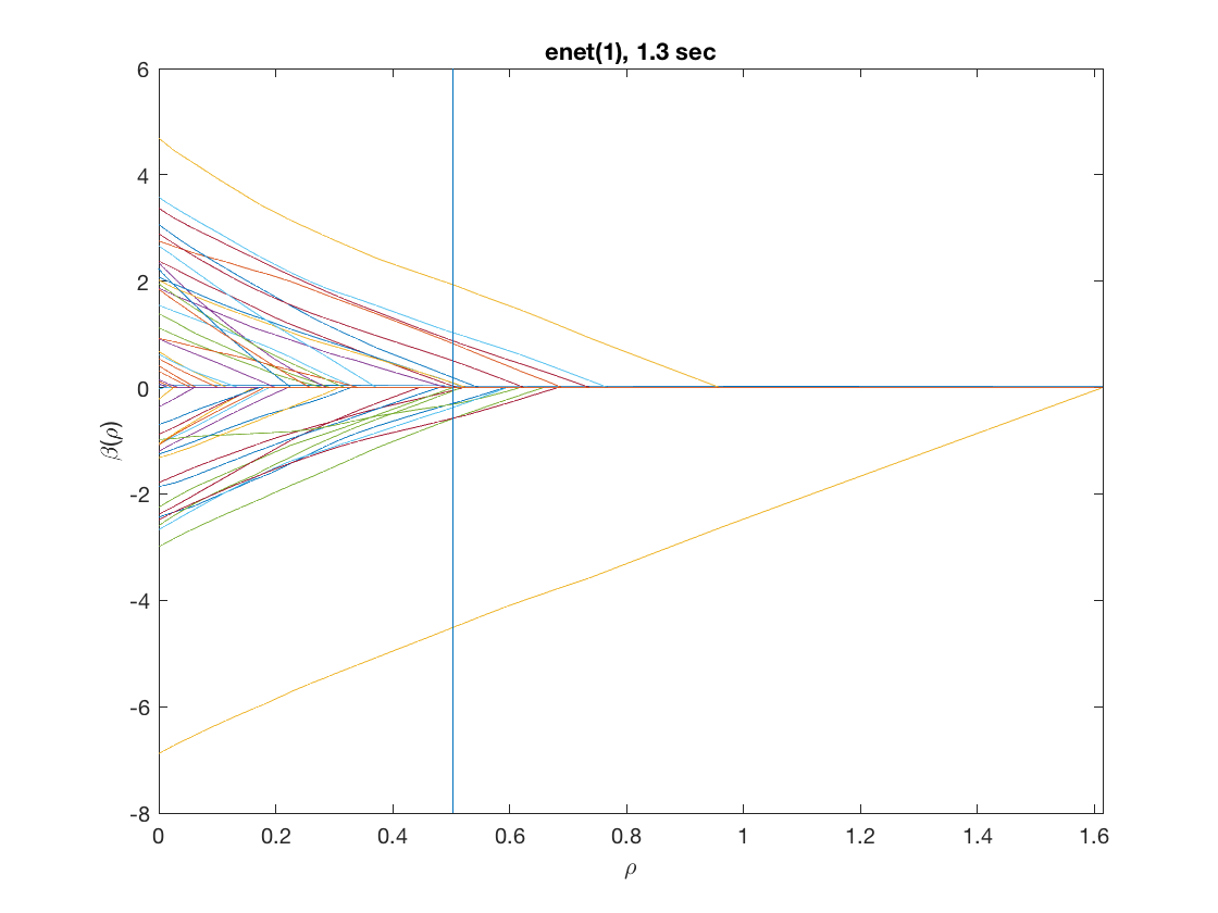
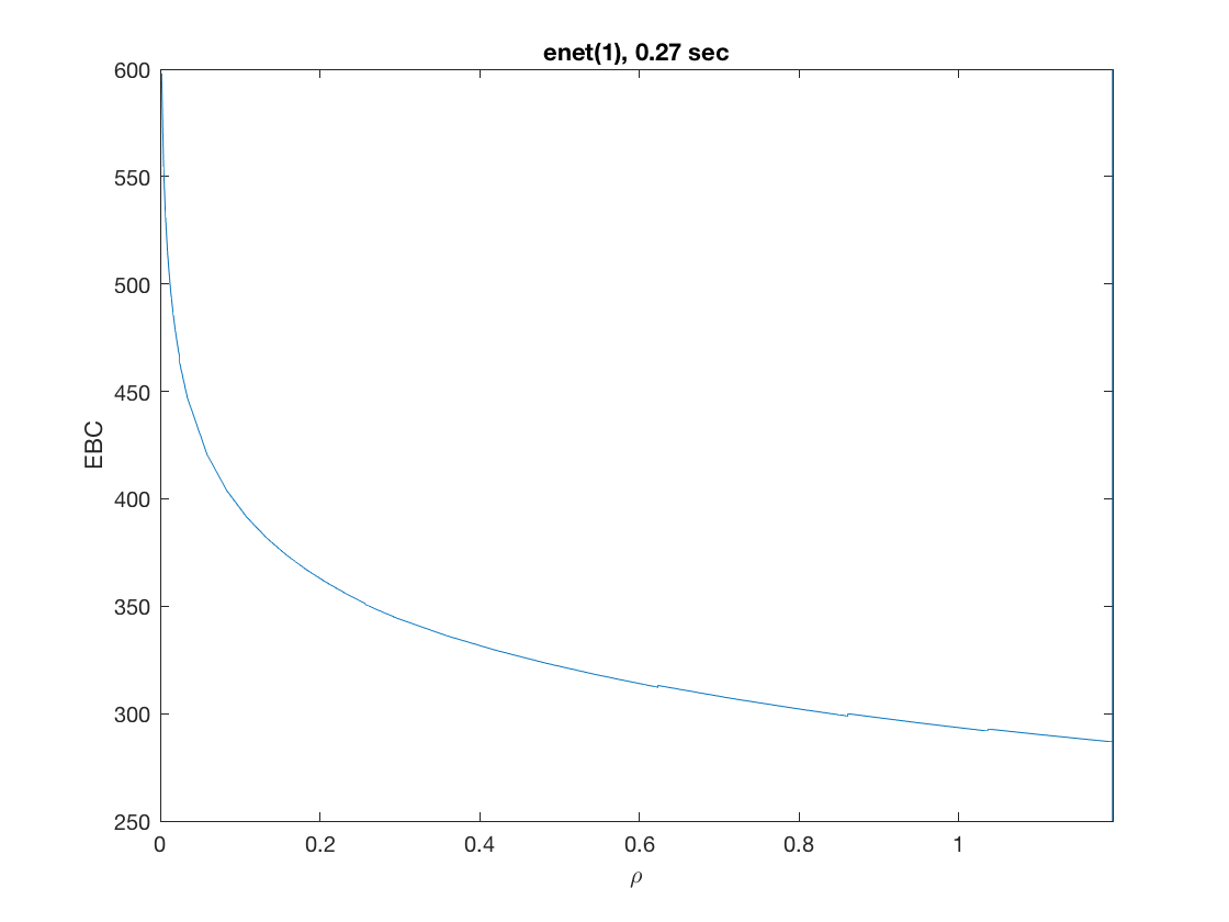
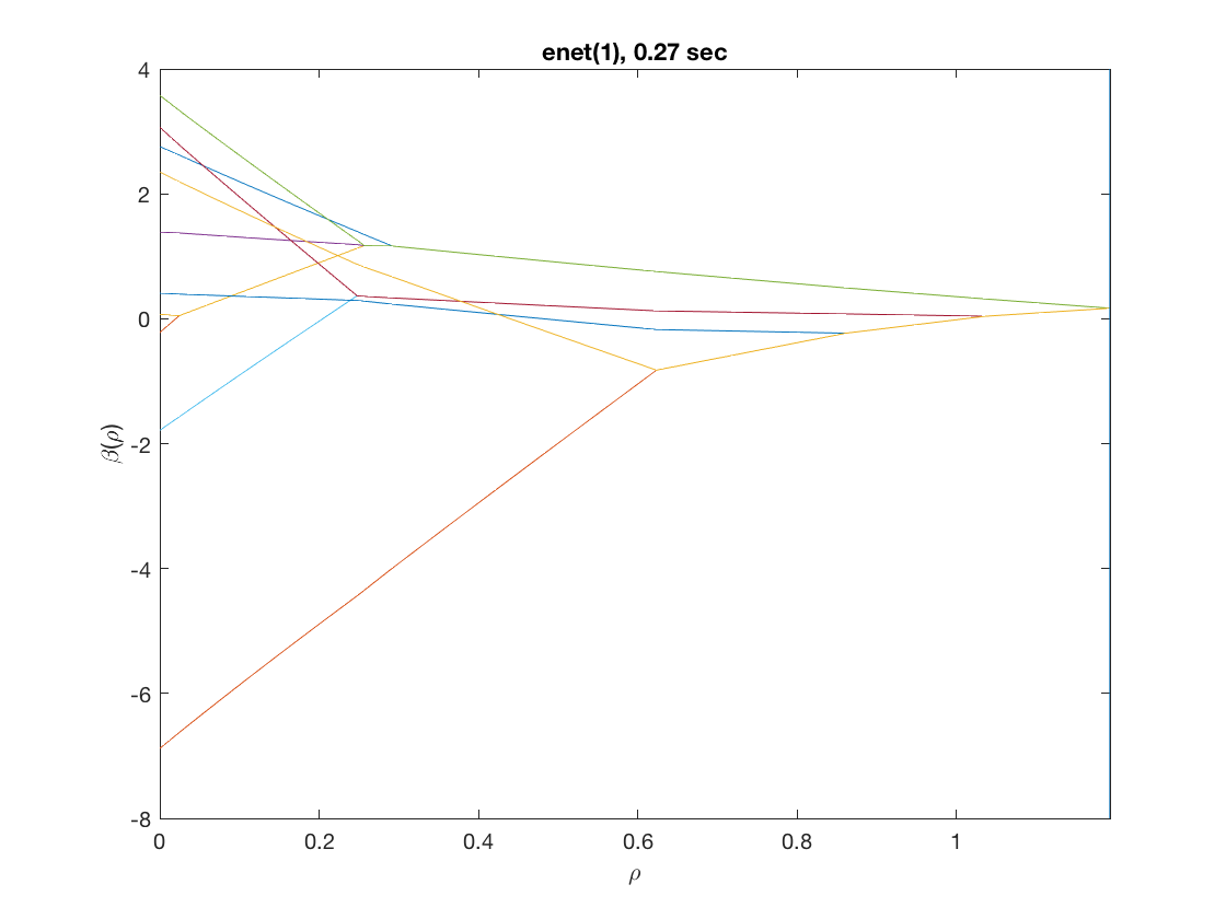
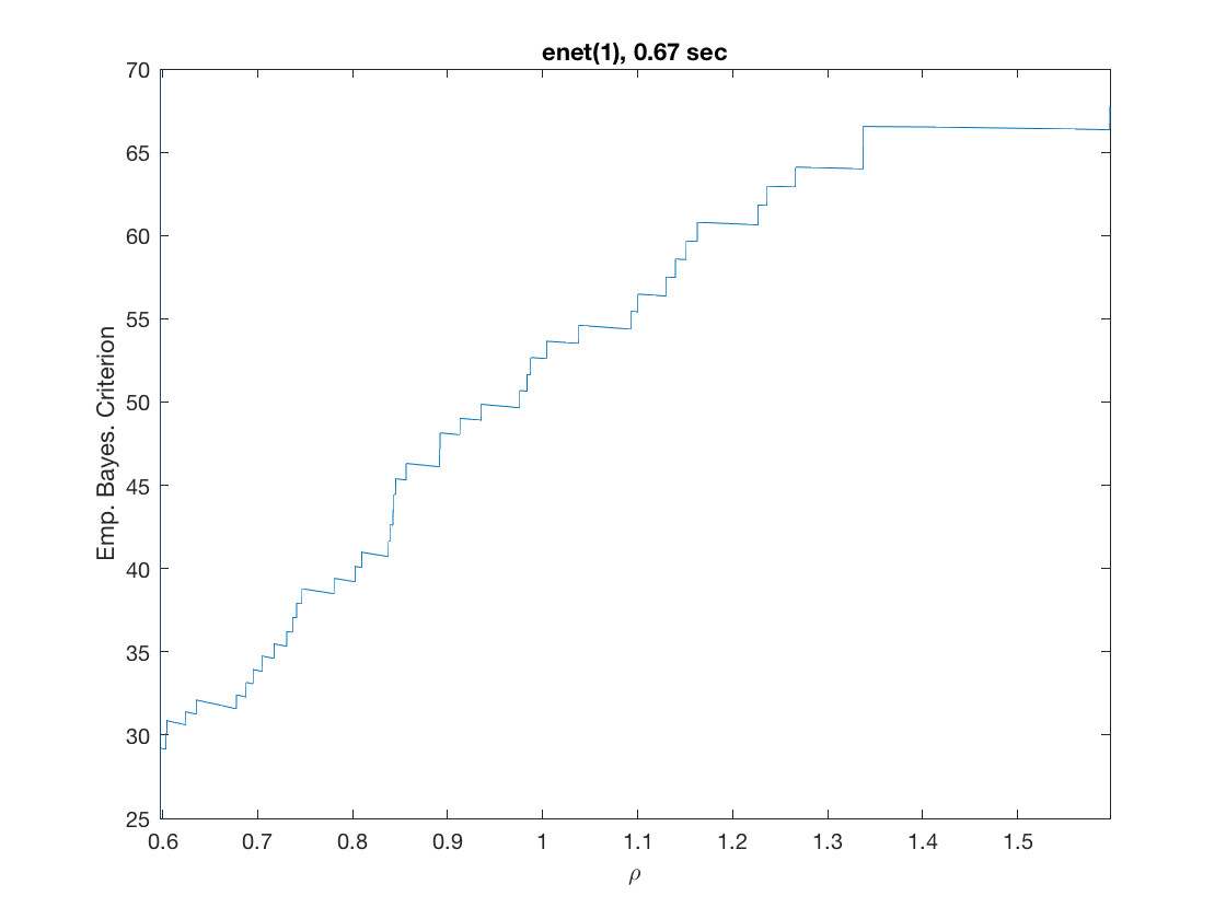
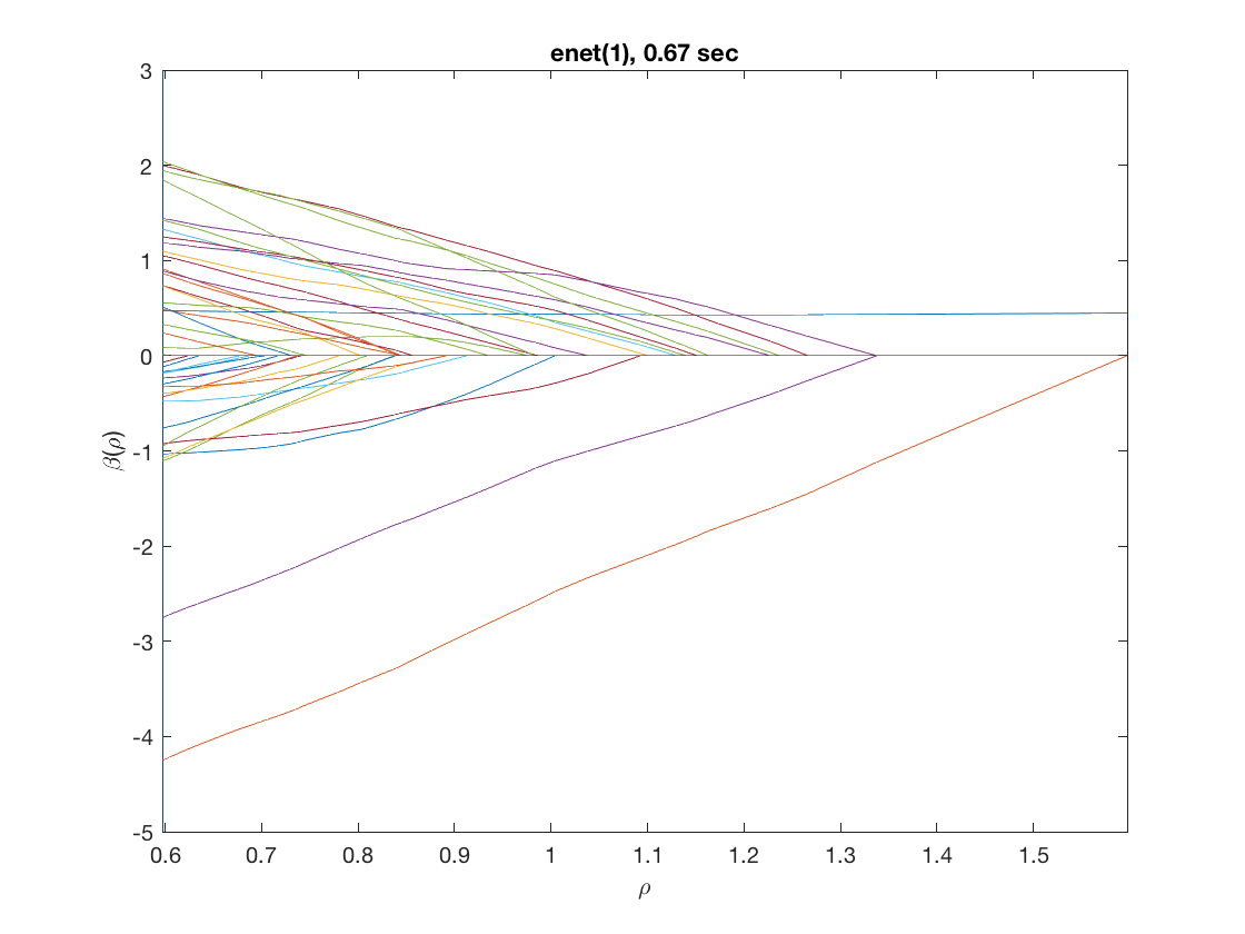
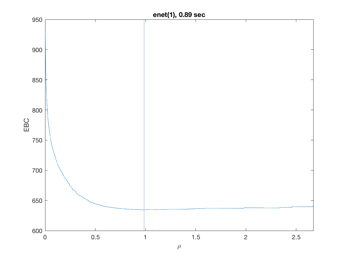
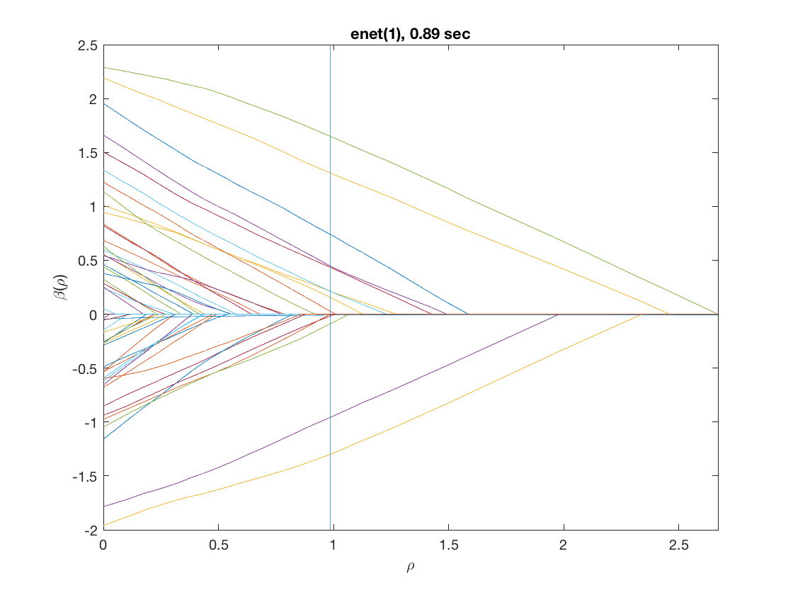
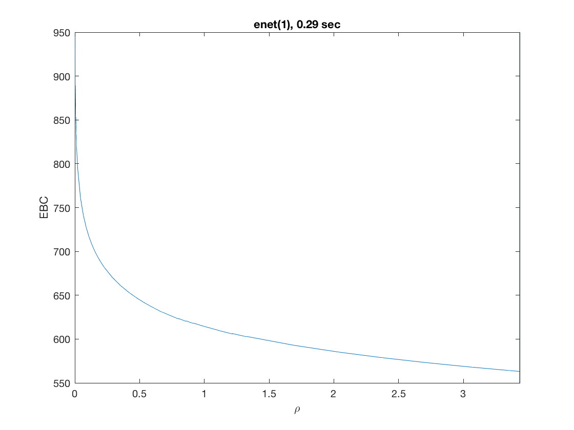
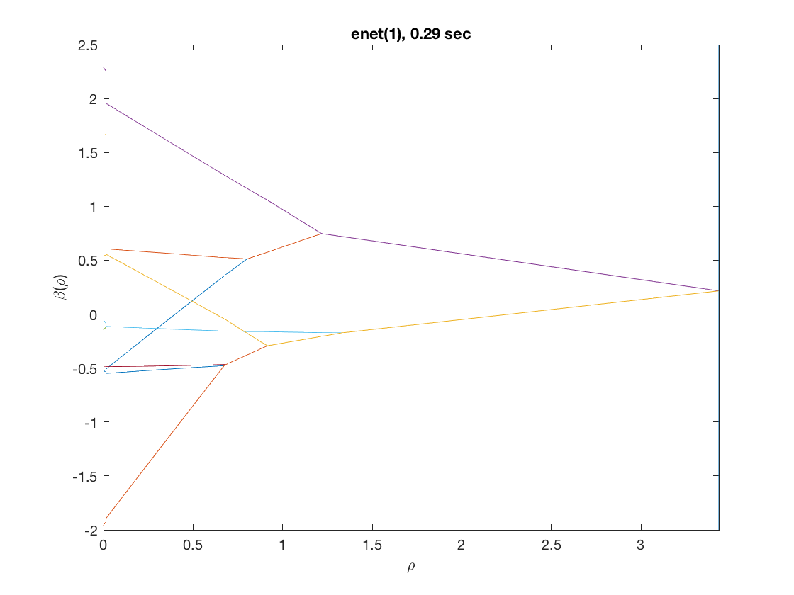
Solution path for lasso

model = 'logistic';         % do logistic regression
penalty = 'enet';           % set penalty to lasso
penparam = 1;
penidx = [false; true(size(X,2)-1,1)]; % leave intercept unpenalized
tic;
[rho_path,beta_path,eb_path] = ...  % compute solution path
    glm_sparsepath(X,y,model,'penidx',penidx,'penalty',penalty, ...
    'penparam',penparam);
timing = toc;
[~,ebidx] = min(eb_path);   % locate the best model by empirical Bayes crit.

figure;
plot(rho_path,eb_path);
xlabel('\rho');
ylabel('Emp. Bayes. Criterion');
xlim([min(rho_path),max(rho_path)]);
title([penalty '(' num2str(penparam) '), ' num2str(timing,2) ' sec']);
line([rho_path(ebidx), rho_path(ebidx)], ylim);

figure;
plot(rho_path,beta_path);
xlabel('\rho');
ylabel('\beta(\rho)');
xlim([min(rho_path),max(rho_path)]);
title([penalty '(' num2str(penparam) '), ' num2str(timing,2) ' sec']);
line([rho_path(ebidx), rho_path(ebidx)], ylim);

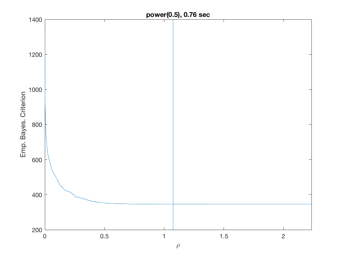
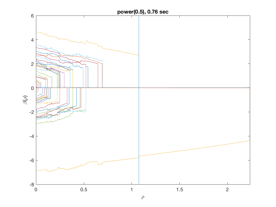
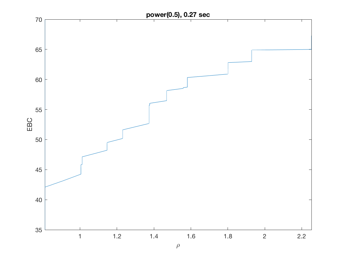
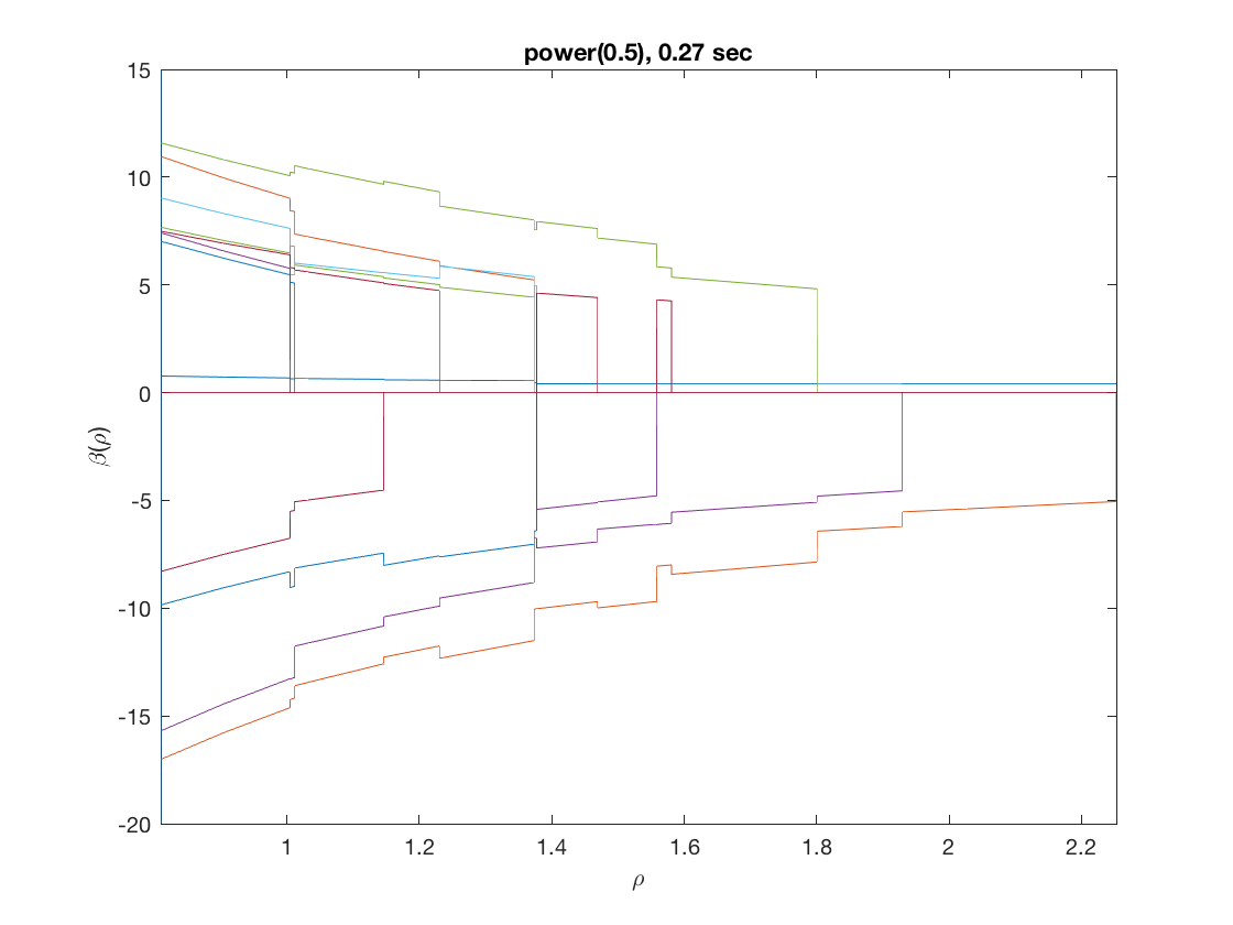
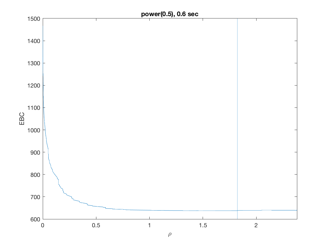
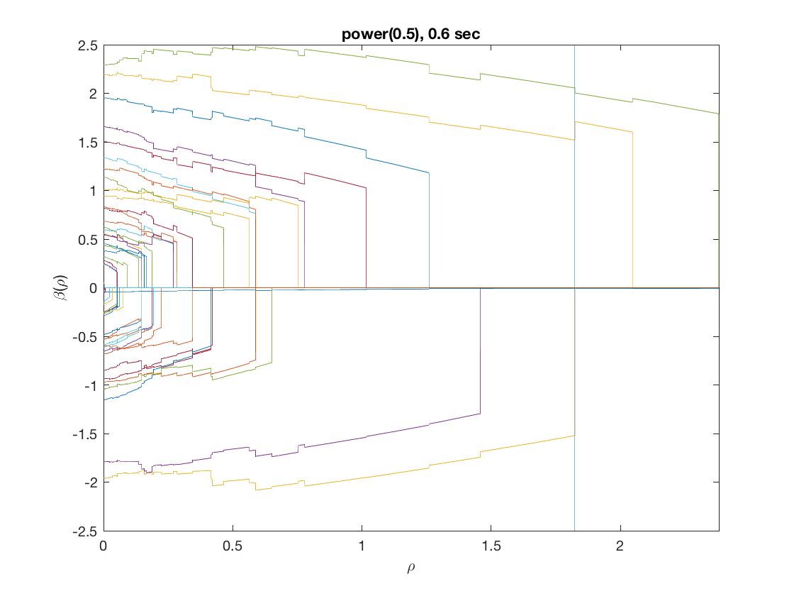
Solution path for power (0.5)

penalty = 'power';          % set penalty function to power
penparam = 0.5;
tic;
[rho_path,beta_path,eb_path] = ...  % compute solution path
    glm_sparsepath(X,y,model,'penidx',penidx,'penalty',penalty, ...
    'penparam',penparam);
timing = toc;
[~,ebidx] = min(eb_path);

figure;
plot(rho_path,eb_path);
xlabel('\rho');
ylabel('Emp. Bayes. Criterion');
xlim([min(rho_path),max(rho_path)]);
title([penalty '(' num2str(penparam) '), ' num2str(timing,2) ' sec']);
line([rho_path(ebidx), rho_path(ebidx)], ylim);

figure;
plot(rho_path,beta_path);
xlabel('\rho');
ylabel('\beta(\rho)');
xlim([min(rho_path),max(rho_path)]);
title([penalty '(' num2str(penparam) '), ' num2str(timing,2) ' sec']);
line([rho_path(ebidx), rho_path(ebidx)], ylim);

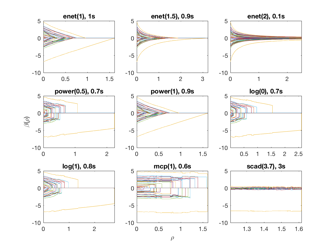
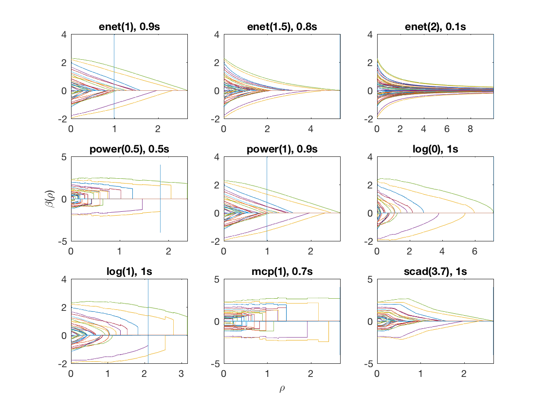
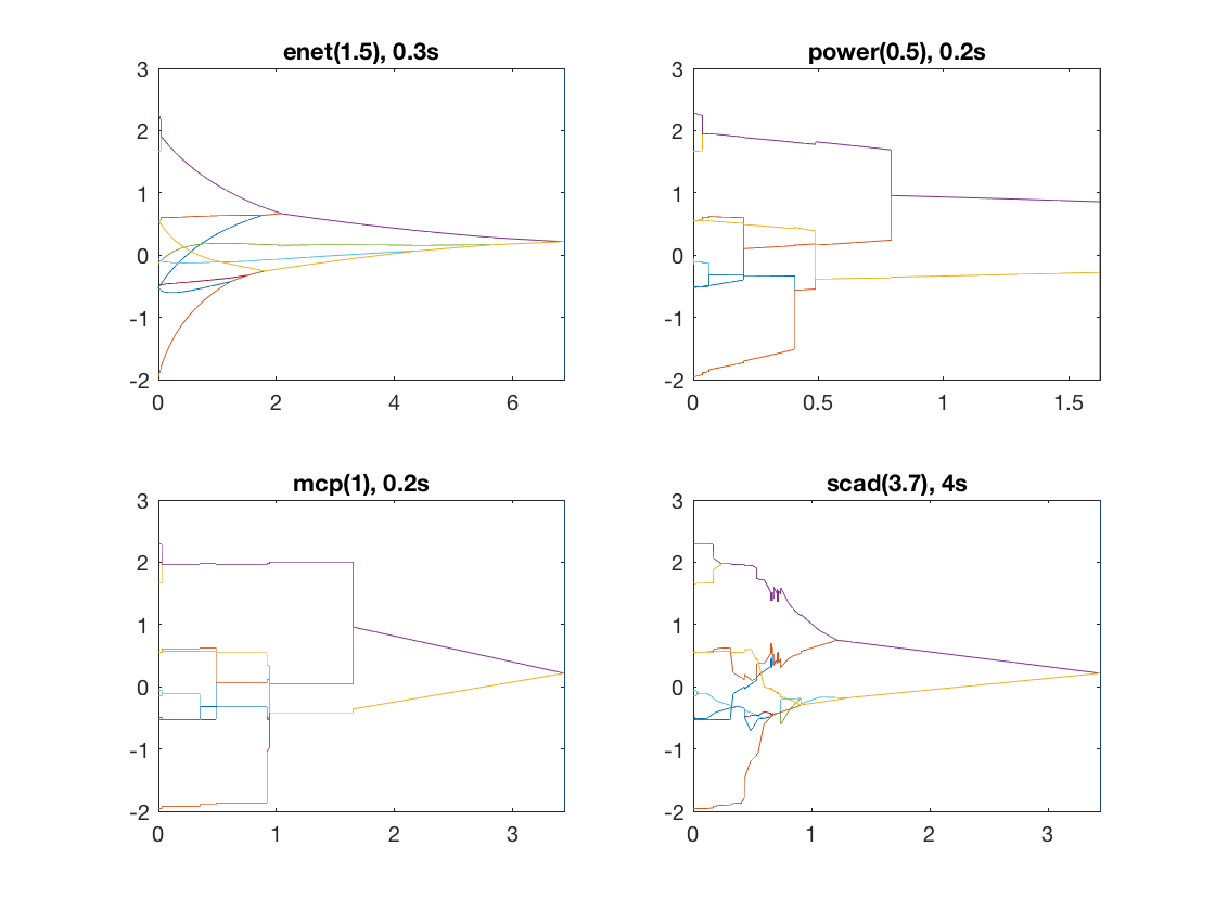
Compare solution paths from different penalties

penalty = {'enet' 'enet' 'enet' 'power' 'power' 'log' 'log' 'mcp' 'scad'};
penparam = [1 1.5 2 0.5 1 0 1 1 3.7];
penidx = [false; true(size(X,2)-1,1)];  % leave intercept unpenalized

figure;
for i=1:length(penalty)
    tic;
    [rho_path,beta_path] = ...
        glm_sparsepath(X,y,model,'penidx',penidx,'penalty',penalty{i}, ...
        'penparam',penparam(i));
    timing = toc;
    subplot(3,3,i);
    plot(rho_path,beta_path);
    if (i==8)
        xlabel('\rho');
    end
    if (i==4)
        ylabel('\beta(\rho)');
    end
    xlim([min(rho_path),max(rho_path)]);
    title([penalty{i} '(' num2str(penparam(i)) '), ' num2str(timing,1) 's']);
end

Fused logistic regression

Fused logistic regression (fusing the first 10 predictors)

D = zeros(9,size(X,2));     % regularization matrix for fusing first 10 preds
D(10:10:90) = 1;
D(19:10:99) = -1;
disp(D(1:9,1:11));
model = 'logistic';
penalty = 'enet';           % set penalty function to lasso
penparam = 1;
tic;
[rho_path,beta_path,eb_path] = glm_regpath(X,y,D,model,'penalty',penalty, ...
    'penparam',penparam);
timing = toc;
[~,ebidx] = min(eb_path);

figure;
plot(rho_path,eb_path);
xlabel('\rho');
ylabel('EBC');
xlim([min(rho_path),max(rho_path)]);
title([penalty '(' num2str(penparam) '), ' num2str(timing,2) ' sec']);
line([rho_path(ebidx), rho_path(ebidx)], ylim);

figure;
plot(rho_path,beta_path(2:11,:));
xlabel('\rho');
ylabel('\beta(\rho)');
xlim([min(rho_path),max(rho_path)]);
title([penalty '(' num2str(penparam) '), ' num2str(timing,2) ' sec']);
line([rho_path(ebidx), rho_path(ebidx)], ylim);

     0     1    -1     0     0     0     0     0     0     0     0
     0     0     1    -1     0     0     0     0     0     0     0
     0     0     0     1    -1     0     0     0     0     0     0
     0     0     0     0     1    -1     0     0     0     0     0
     0     0     0     0     0     1    -1     0     0     0     0
     0     0     0     0     0     0     1    -1     0     0     0
     0     0     0     0     0     0     0     1    -1     0     0
     0     0     0     0     0     0     0     0     1    -1     0
     0     0     0     0     0     0     0     0     0     1    -1

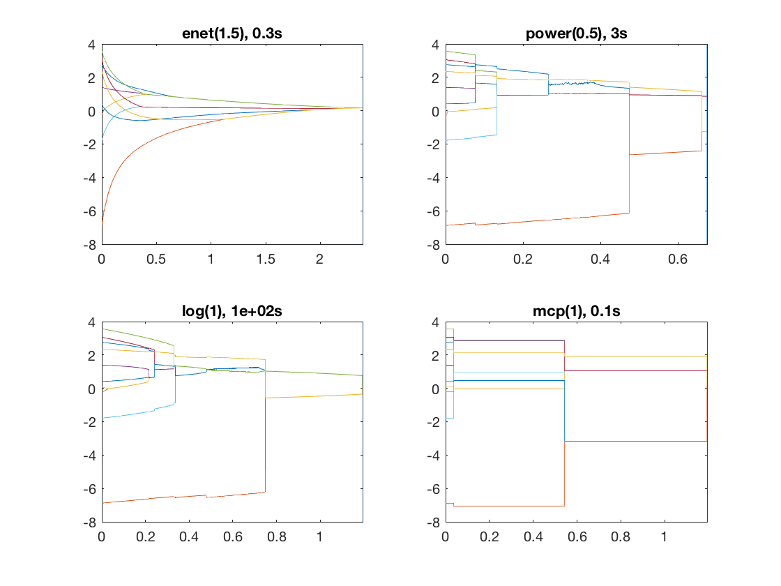
Same fusion problem, but with power, log, MCP, and SCAD penalty

penalty = {'enet' 'power' 'log' 'mcp'};
penparam = [1.5 0.5 1 1];
for i=1:length(penalty)
    disp(penalty(i))
    tic;
    [rho_path, beta_path,eb_path] = glm_regpath(X,y,D,model,'penalty',penalty{i},...
        'penparam',penparam(i));
    timing = toc;
    [~,ebidx] = min(eb_path);
    subplot(2,2,i);
    plot(rho_path,beta_path(2:11,:));
    xlim([min(rho_path),max(rho_path)]);
    title([penalty{i} '(' num2str(penparam(i)) '), ' num2str(timing,1) 's']);
    line([rho_path(ebidx), rho_path(ebidx)], ylim);
end

    'enet'

    'power'

Warning: Matrix is close to singular or badly scaled. Results may be inaccurate.
RCOND =  8.158071e-21. 
    'log'

    'mcp'

Sparse logistic regression (n<p)

Simulate another sample data set (n=100, p=1000)

clear;
n = 100;
p = 1000;
X = randn(n,p);             % generate a random design matrix
X = bsxfun(@rdivide, X, sqrt(sum(X.^2,1))); % normalize predictors
X = [ones(size(X,1),1),X];  % add intercept
b = zeros(p+1,1);           % true signal
b(2:6) = 5;                 % first 5 predictors are 5
b(7:11) = -5;               % next 5 predictors are -5
inner = X*b;                % linear parts
prob = 1./(1+exp(-inner));
y = binornd(1,prob);        % generate binary response

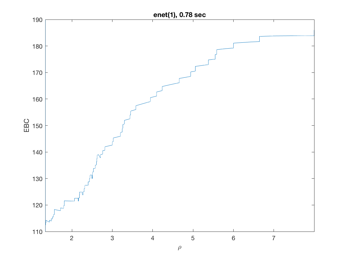
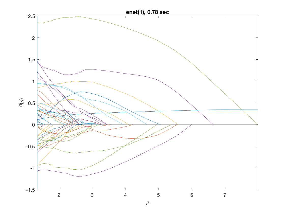
Solution path for lasso

maxpreds = 51;              % request path to the first 51 predictors
model = 'logistic';         % do logistic regression
penalty = 'enet';           % set penalty to lasso
penparam = 1;
penidx = [false; true(size(X,2)-1,1)]; % leave intercept unpenalized
tic;
[rho_path,beta_path,eb_path] = ...  % compute solution path
    glm_sparsepath(X,y,model,'penidx',penidx,'maxpreds',maxpreds, ...
    'penalty',penalty,'penparam',penparam);
timing = toc;
[~,ebidx] = min(eb_path);

figure;
plot(rho_path,eb_path);
xlabel('\rho');
ylabel('Emp. Bayes. Criterion');
xlim([min(rho_path),max(rho_path)]);
title([penalty '(' num2str(penparam) '), ' num2str(timing,2) ' sec']);
line([rho_path(ebidx), rho_path(ebidx)], ylim);

figure;
plot(rho_path,beta_path);
xlabel('\rho');
ylabel('\beta(\rho)');
xlim([min(rho_path),max(rho_path)]);
title([penalty '(' num2str(penparam) '), ' num2str(timing,2) ' sec']);
line([rho_path(ebidx), rho_path(ebidx)], ylim);

Warning: separation detected; perfect prediction achieved

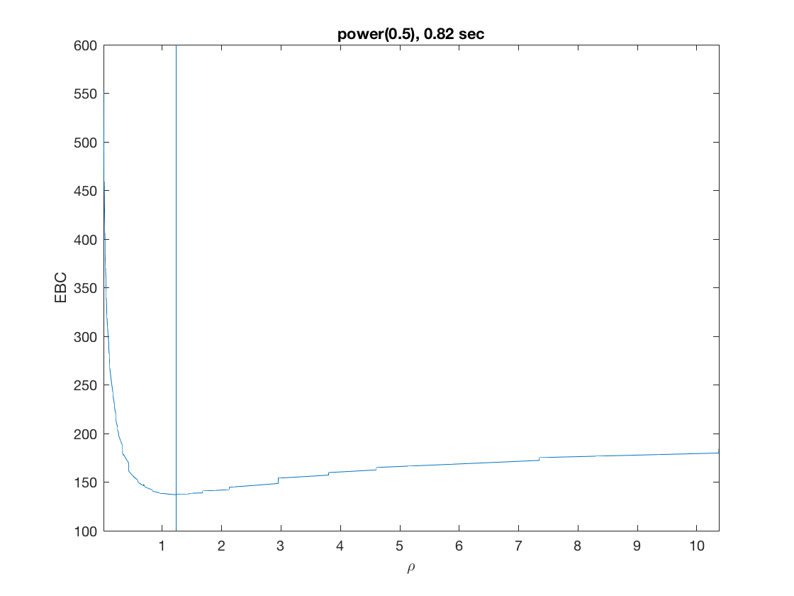
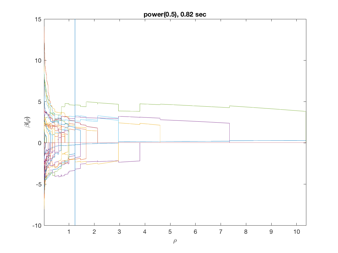
Solution path for power (0.5)

penalty = 'power';          % set penalty function to power
penparam = 0.5;
tic;
[rho_path,beta_path,eb_path] = ...  % compute solution path
    glm_sparsepath(X,y,model,'penidx',penidx,'maxpreds',maxpreds, ...
    'penalty',penalty,'penparam',penparam);
timing = toc;
[~,ebidx] = min(eb_path);

figure;
plot(rho_path,eb_path);
xlabel('\rho');
ylabel('EBC');
xlim([min(rho_path),max(rho_path)]);
title([penalty '(' num2str(penparam) '), ' num2str(timing,2) ' sec']);
line([rho_path(ebidx), rho_path(ebidx)], ylim);

figure;
plot(rho_path,beta_path);
xlabel('\rho');
ylabel('\beta(\rho)');
xlim([min(rho_path),max(rho_path)]);
title([penalty '(' num2str(penparam) '), ' num2str(timing,2) ' sec']);
line([rho_path(ebidx), rho_path(ebidx)], ylim);

Warning: separation detected; perfect prediction achieved

Sparse loglinear (Poisson) regression (n>p)

Simulate a sample data set (n=500, p=50)

clear;
n = 500;
p = 50;
X = randn(n,p);             % generate a random design matrix
X = bsxfun(@rdivide, X, sqrt(sum(X.^2,1))); % normalize predictors
X = [ones(size(X,1),1) X];  % add intercept
b = zeros(p+1,1);           % true signal: first ten predictors are 3
b(2:6) = 1;                 % first 5 predictors are 1
b(7:11) = -1;               % next 5 predictors are -1
inner = X*b;                % linear parts
y = poissrnd(exp(inner));   % generate response from Poisson

Sparse loglinear regression at a fixed tuning parameter value

model = 'loglinear';        % set model to logistic
penidx = [false; true(size(X,2)-1,1)];  % leave intercept unpenalized
penalty = 'enet';           % set penalty to lasso
penparam = 1;
lambdastart = 0;            % find the maximum tuning parameter to start
for j=1:size(X,2)
    if (penidx(j))
    lambdastart = max(lambdastart, ...
        glm_maxlambda(X(:,j),y,model,'penalty',penalty,'penparam',penparam));
    end
end
disp(lambdastart);

lambda = 0.9*lambdastart;   % tuning parameter value
betahat = ...               % sparse regression
    glm_sparsereg(X,y,lambda,model,'penidx',penidx,'penalty',penalty, ...
    'penparam',penparam);

figure;                     % plot penalized estimate
bar(1:length(betahat),betahat);
xlabel('j');
ylabel('\beta_j');
xlim([0,length(betahat)+1]);
title([penalty '(' num2str(penparam) '), \lambda=' num2str(lambda,2)]);

lambda = 0.5*lambdastart;   % tuning parameter value
betahat = ...               % sparse regression
    glm_sparsereg(X,y,lambda,model,'penidx',penidx,'penalty',penalty, ...
    'penparam',penparam);

figure;                     % plot penalized estimate
bar(1:length(betahat),betahat);
xlabel('j');
ylabel('\beta_j');
xlim([0,length(betahat)+1]);
title([penalty '(' num2str(penparam) '), \lambda=' num2str(lambda,2)]);

    2.6733

Solution path for lasso

model = 'loglinear';        % do logistic regression
penalty = 'enet';           % set penalty to lasso
penparam = 1;
penidx = [false; true(size(X,2)-1,1)]; % leave intercept unpenalized
tic;
[rho_path,beta_path,eb_path] = ...  % compute solution path
    glm_sparsepath(X,y,model,'penidx',penidx,'penalty',penalty, ...
    'penparam',penparam);
timing = toc;
[~,ebidx] = min(eb_path);

figure;
plot(rho_path,eb_path);
xlabel('\rho');
ylabel('EBC');
xlim([min(rho_path),max(rho_path)]);
title([penalty '(' num2str(penparam) '), ' num2str(timing,2) ' sec']);
line([rho_path(ebidx), rho_path(ebidx)], ylim);

figure;
plot(rho_path,beta_path);
xlabel('\rho');
ylabel('\beta(\rho)');
xlim([min(rho_path),max(rho_path)]);
title([penalty '(' num2str(penparam) '), ' num2str(timing,2) ' sec']);
line([rho_path(ebidx), rho_path(ebidx)], ylim);

Solution path for power (0.5)

penalty = 'power';          % set penalty function to power
penparam = 0.5;
tic;
[rho_path,beta_path,eb_path] = ...  % compute solution path
    glm_sparsepath(X,y,model,'penidx',penidx,'penalty',penalty, ...
    'penparam',penparam);
timing = toc;
[~,ebidx] = min(eb_path);

figure;
plot(rho_path,eb_path);
xlabel('\rho');
ylabel('EBC');
xlim([min(rho_path),max(rho_path)]);
title([penalty '(' num2str(penparam) '), ' num2str(timing,2) ' sec']);
line([rho_path(ebidx), rho_path(ebidx)], ylim);

figure;
plot(rho_path,beta_path);
xlabel('\rho');
ylabel('\beta(\rho)');
xlim([min(rho_path),max(rho_path)]);
title([penalty '(' num2str(penparam) '), ' num2str(timing,2) ' sec']);
line([rho_path(ebidx), rho_path(ebidx)], ylim);

Compare solution paths from different penalties

penalty = {'enet' 'enet' 'enet' 'power' 'power' 'log' 'log' 'mcp' 'scad'};
penparam = [1 1.5 2 0.5 1 0 1 1 3.7];
penidx = [false; true(size(X,2)-1,1)];  % leave intercept unpenalized

figure;
for i=1:length(penalty)
    disp(penalty(i));
    tic;
    [rho_path,beta_path,eb_path] = glm_sparsepath(X,y,model,'penidx',penidx, ...
        'penalty',penalty{i},'penparam',penparam(i));
    timing = toc;
    [~,ebidx] = min(eb_path);
    subplot(3,3,i);
    plot(rho_path,beta_path);
    if (i==8)
        xlabel('\rho');
    end
    if (i==4)
        ylabel('\beta(\rho)');
    end
    xlim([min(rho_path),max(rho_path)]);
    title([penalty{i} '(' num2str(penparam(i)) '), ' num2str(timing,1) 's']);
    line([rho_path(ebidx), rho_path(ebidx)], ylim);
end

    'enet'

    'enet'

    'enet'

    'power'

    'power'

    'log'

    'log'

    'mcp'

    'scad'

Fused loglinear (Poisson) regression

Fused loglinear regression (fusing the first 10 predictors)

D = zeros(9,size(X,2));     % regularization matrix for fusing first 10 preds
D(10:10:90) = 1;
D(19:10:99) = -1;
disp(D(1:9,1:11));
model = 'loglinear';
penalty = 'enet';          % set penalty function to lasso
penparam = 1;
tic;
[rho_path,beta_path,eb_path] = glm_regpath(X,y,D,model,'penalty',penalty, ...
    'penparam',penparam);
timing = toc;
[~,ebidx] = min(eb_path);

figure;
plot(rho_path,eb_path);
xlabel('\rho');
ylabel('EBC');
xlim([min(rho_path),max(rho_path)]);
title([penalty '(' num2str(penparam) '), ' num2str(timing,2) ' sec']);
line([rho_path(ebidx), rho_path(ebidx)], ylim);

figure;
plot(rho_path,beta_path(2:11,:));
xlabel('\rho');
ylabel('\beta(\rho)');
xlim([min(rho_path),max(rho_path)]);
title([penalty '(' num2str(penparam) '), ' num2str(timing,2) ' sec']);
line([rho_path(ebidx), rho_path(ebidx)], ylim);

     0     1    -1     0     0     0     0     0     0     0     0
     0     0     1    -1     0     0     0     0     0     0     0
     0     0     0     1    -1     0     0     0     0     0     0
     0     0     0     0     1    -1     0     0     0     0     0
     0     0     0     0     0     1    -1     0     0     0     0
     0     0     0     0     0     0     1    -1     0     0     0
     0     0     0     0     0     0     0     1    -1     0     0
     0     0     0     0     0     0     0     0     1    -1     0
     0     0     0     0     0     0     0     0     0     1    -1

Same fusion problem, but with enet, power, MCP, and SCAD penalty

penalty = {'enet' 'power' 'mcp' 'scad'};
penparam = [1.5 0.5 1 3.7];
for i=1:length(penalty)
    disp(penalty(i));
    tic;
    [rho_path,beta_path,eb_path] = glm_regpath(X,y,D,model,'penalty',penalty{i}, ...
        'penparam',penparam(i));
    timing = toc;
    [~,ebidx] = min(eb_path);
    subplot(2,2,i);
    plot(rho_path,beta_path(2:11,:));
    xlim([min(rho_path),max(rho_path)]);
    title([penalty{i} '(' num2str(penparam(i)) '), ' num2str(timing,1) 's']);
    line([rho_path(ebidx), rho_path(ebidx)], ylim);
end

    'enet'

    'power'

    'mcp'

    'scad'

Sparse loglinear (Poisson) regression (n<<p)

Simulate a sample data set (n=500, p=50)

clear;
n = 100;
p = 1000;
X = randn(n,p);             % generate a random design matrix
X = bsxfun(@rdivide, X, sqrt(sum(X.^2,1))); % normalize predictors
X = [ones(size(X,1),1) X];  % add intercept
b = zeros(p+1,1);           % true signal: first ten predictors are 3
b(2:6) = 3;                 % first 5 predictors are 3
b(7:11) = -3;               % next 5 predictors are -3
inner = X*b;                % linear parts
y = poissrnd(exp(inner));   % generate response from Poisson

Solution path for lasso

maxpreds = 51;              % obtain solution path to top 50 predictors
model = 'loglinear';        % do Poisson regression
penalty = 'enet';           % set penalty to lasso
penparam = 1;
penidx = [false; true(size(X,2)-1,1)]; % leave intercept unpenalized
tic;
[rho_path,beta_path,eb_path] = ...  % compute solution path
    glm_sparsepath(X,y,model,'penidx',penidx,'penalty',penalty, ...
    'penparam',penparam,'maxpreds',maxpreds);
timing = toc;
[~,ebidx] = min(eb_path);

figure;
plot(rho_path,eb_path);
xlabel('\rho');
ylabel('EBC');
xlim([min(rho_path),max(rho_path)]);
title([penalty '(' num2str(penparam) '), ' num2str(timing,2) ' sec']);
line([rho_path(ebidx), rho_path(ebidx)], ylim);

figure;
plot(rho_path,beta_path);
xlabel('\rho');
ylabel('\beta(\rho)');
xlim([min(rho_path),max(rho_path)]);
title([penalty '(' num2str(penparam) '), ' num2str(timing,2) ' sec']);
line([rho_path(ebidx), rho_path(ebidx)], ylim);

Solution path for power (0.5)

penalty = 'power';          % set penalty function to power
penparam = 0.5;
tic;
[rho_path,beta_path,eb_path] = ...  % compute solution path
    glm_sparsepath(X,y,model,'penidx',penidx,'penalty',penalty, ...
    'penparam',penparam,'maxpreds',maxpreds);
timing = toc;
[~,ebidx] = min(eb_path);

figure;
plot(rho_path,eb_path);
xlabel('\rho');
ylabel('EBC');
xlim([min(rho_path),max(rho_path)]);
title([penalty '(' num2str(penparam) '), ' num2str(timing,2) ' sec']);
line([rho_path(ebidx), rho_path(ebidx)], ylim);

figure;
plot(rho_path,beta_path);
xlabel('\rho');
ylabel('\beta(\rho)');
xlim([min(rho_path),max(rho_path)]);
title([penalty '(' num2str(penparam) '), ' num2str(timing,2) ' sec']);
line([rho_path(ebidx), rho_path(ebidx)], ylim);

Sparse generalized linear model (GLM)

Contents

Sparse logistic regression (n>p)

Fused logistic regression

Sparse logistic regression (n<p)

Sparse loglinear (Poisson) regression (n>p)

Fused loglinear (Poisson) regression

Sparse loglinear (Poisson) regression (n<<p)