Introduction to ...
![]()
Types of computer languages
Compiled languages: C/C++, Fortran, ...
- Directly compiled to machine code that is executed by CPU
- Pros: fast, memory efficient
- Cons: longer development time, hard to debug
Interpreted language: R, Matlab, SAS IML, JavaScript, BASIC, ...
- Interpreted by interpreter
- Pros: fast prototyping
- Cons: excruciatingly slow for loops
Mixed (dynamic) languages: Julia, Python, JAVA, Matlab (JIT), R (
compilerpackage), ...- Dynamic is versus to the static compiled languages
- Pros and cons: between the compiled and interpreted languages
Script languages: Linux shell scripts, Perl, ...
- Extremely useful for some data preprocessing and manipulation
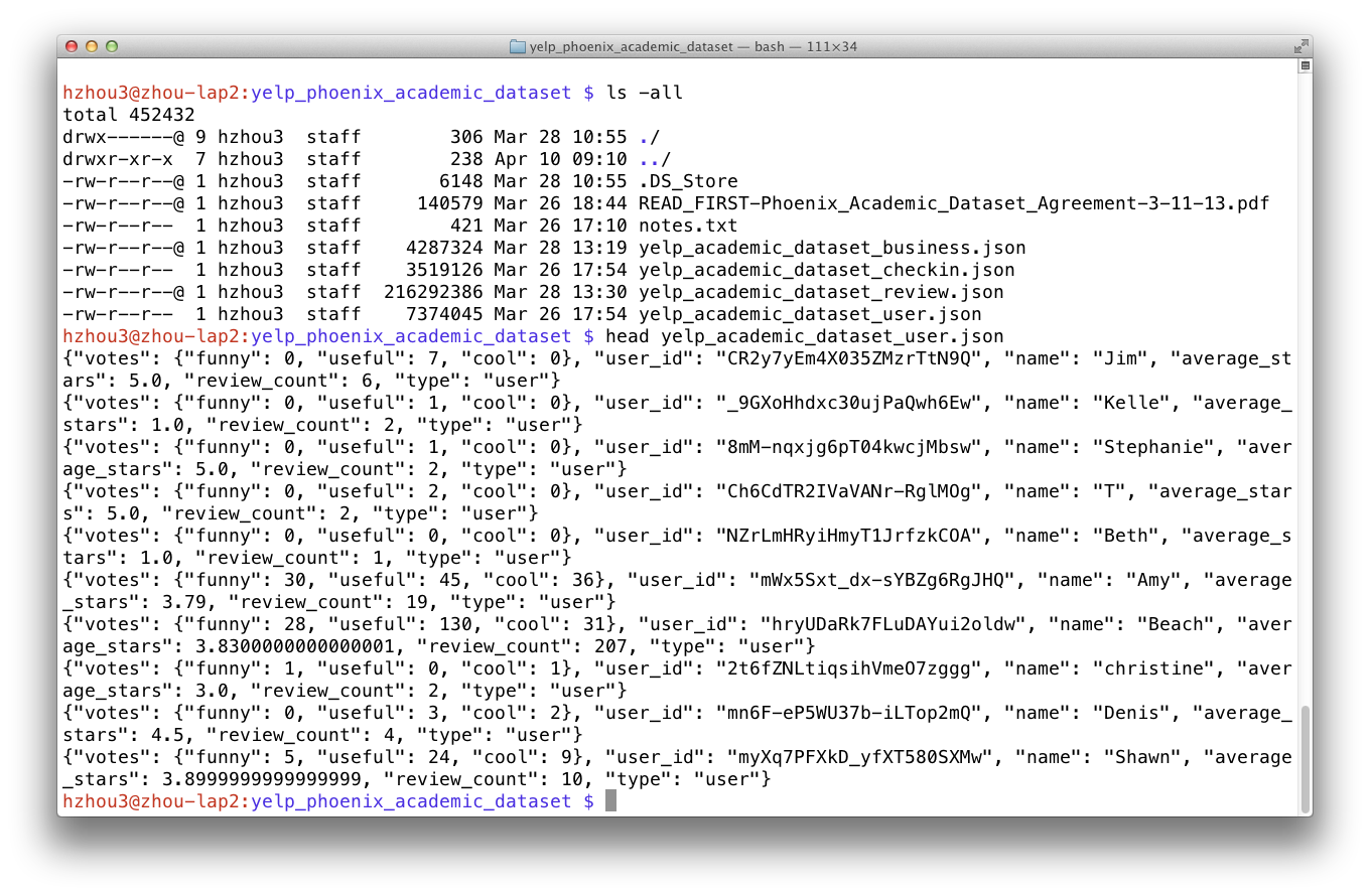
- E.g., massage the Yelp data before analysis
- Database languages: SQL, Hadoop.
- Data analysis never happens if we do not know how to retrieve data from databases
Messages
To be versatile in the big data era, master at least one language in each category.
To improve efficiency of interpreted languages such as R or Matlab, conventional wisdom is to avoid loops as much as possible. Aka, vectorize code
The only loop you are allowed to have is that for an iterative algorithm.
For some tasks where looping is necessary, consider coding in C or Fortran. It is "convenient" to incorporate compiled code into R or Matlab. But do this only after profiling.
Success stories:glmnetpackages in R is coded in Fortran.Modern languages such as Julia tries to solve the two language problem. That is to achieve efficiency without vectorizing code.
What's Julia?
Julia is a high-level, high-performance dynamic programming language for technical computing, with syntax that is familiar to users of other technical computing environments
Started in 2009. First public release in 2012.
- Creators: Jeff Bezanson, Alan Edelman, Stefan Karpinski, Viral Shah
- Current release v0.5.1
- v1.0 is staged to release in 2017
Aims to solve the notorious "two language problem":
- Prototype code goes into high-level languages like R/Python, production code goes into low-level language like C/C++
Write high-level, abstract code that closely resembles mathematical formulas
- yet produces fast, low-level machine code that has traditionally only been generated by static languages.
Julia is more than just "Fast R" or "Fast Matlab"
- Performance comes from features that work well together.
- You can't just take the magic dust that makes Julia fast and sprinkle it on [language of choice]
R is great, but...
It's not meant for high performance computing
- http://adv-r.had.co.nz/Performance.html
- Section on performance starts with "Why is R slow?"
- http://adv-r.had.co.nz/Performance.html
Deficiencies in the core language
- Some fixed with packages (
devtools,roxygen2,Matrix) - Others harder to fix (R uses an old version of BLAS)
- Some impossible to fix (clunky syntax, poor design choices)
- Some fixed with packages (
Only 6 active developers left (out of 20 R-Core members)
- JuliaLang organization has 74 members, with 567 total contributors (as of 3/3/17)
Doug Bates (member of R-Core,
Matrixandlme4)- Getting Doug on board was a big win for statistics with Julia, as he brought a lot of knowledge about the history of R development and design choices
https://github.com/dmbates/MixedModels.jl
As some of you may know, I have had a (rather late) mid-life crisis and run off with another language called Julia.
-- Doug Bates (on the `knitr` Google Group)
Language features of R, Matlab and Julia
| Features | R | Matlab | Julia |
|---|---|---|---|
| Open source | 👍 | 👎 | 👍 |
| IDE | RStudio 👍 👍 | 👍 👍 👍 | Atom+Juno 👎 |
| Dynamic document | RMarkdown 👍 👍 👍 | 👍 👍 | IJulia 👍 👍 |
| Multi-threading | parallel 👎 |
👍 | 👍 👍 see docs |
| JIT | compiler 👎 |
👍 👍 | 👍 👍 👍 |
| Call C/Fortran | wrapper, Rcpp |
wrapper | no glue code needed |
| Call shared library | wrapper | wrapper | no glue code needed |
| Type system | 👎 | 👍 👍 | 👍 👍 👍 |
| Pass by reference | 👎 | 👎 | 👍 👍 👍 |
| Linear algebra | 👎 | MKL, Arpack | OpenBLAS, eigpack |
| Distributed computing | 👎 | 👍 | 👍 👍 👍 |
| Sparse linear algebra | Matrix package 👎 |
👍 👍 👍 | 👍 👍 👍 |
| Documentation | 👎 | 👍 👍 👍 | 👍 👍 |
| Profiler | 👎 | 👍 👍 👍 | 👍 👍 👍 |
Benchmark
Benchmark code
R-benchmark-25.Rfrom http://r.research.att.com/benchmarks/R-benchmark-25.R covers many commonly used numerical operations used in statistics.We ported (literally) to Matlab and Julia and report the run times (averaged over 5 runs) here.
| Test | R 3.3.2 | Matlab R2017a | Julia 0.5.1 |
|---|---|---|---|
| Matrix creation, trans., deform. (2500 x 2500) | 0.70 | 0.13 | 0.22 |
Power of matrix (2500 x 2500, A.^1000) |
0.17 | 0.10 | 0.11 |
| Quick sort ($n = 7 \times 10^6$) | 0.69 | 0.30 | 0.62 |
| Cross product (2800 x 2800, $A^TA$) | 13.49 | 0.18 | 0.21 |
| LS solution ($n = p = 2000$) | 6.42 | 0.07 | 0.07 |
| FFT ($n = 2,400,000$) | 0.25 | 0.03 | 0.16 |
| Eigen-values ($600 \times 600$) | 0.71 | 0.22 | 0.51 |
| Determinant ($2500 \times 2500$) | 3.49 | 0.19 | 0.14 |
| Cholesky ($3000 \times 3000$) | 5.03 | 0.08 | 0.16 |
| Matrix inverse ($1600 \times 1600$) | 2.83 | 0.11 | 0.18 |
| Fibonacci (vector calculation) | 0.22 | 0.16 | 0.58 |
| Hilbert (matrix calculation) | 0.21 | 0.07 | 0.06 |
| GCD (recursion) | 0.33 | 0.09 | 0.13 |
| Toeplitz matrix (loops) | 0.28 | 0.0012 | 0.0007 |
| Escoufiers (mixed) | 0.33 | 0.15 | 0.14 |
Machine specs: Intel i7 @ 2.9GHz (4 physical cores, 8 threads), 16G RAM, Mac OS 10.12.3.
Gibbs sampler example by Doug Bates
An example from Dr. Doug Bates's slides Julia for R Programmers.
The task is to create a Gibbs sampler for the density
$$ f(x, y) = k x^2 exp(- x y^2 - y^2 + 2y - 4x), x > 0 $$ using the conditional distributions $$ \begin{eqnarray*} X | Y &\sim& \Gamma \left( 3, \frac{1}{y^2 + 4} \right) \\ Y | X &\sim& N \left(\frac{1}{1+x}, \frac{1}{2(1+x)} \right). \end{eqnarray*} $$This is a Julia function for the simple Gibbs sampler:
using Distributions

function jgibbs(N, thin)
    mat = zeros(N, 2)
    x = y = 0.0
    for i in 1:N
        for j in 1:thin
            x = rand(Gamma(3.0, 1.0 / (y * y + 4.0)))
            y = rand(Normal(1.0 / (x + 1.0), 1.0 / sqrt(2.0(x + 1.0))))
        end
        mat[i, 1] = x
        mat[i, 2] = y
    end
    mat
end
Generate a bivariate sample of size 10,000 with a thinning of 500. How long does it take?
jgibbs(100, 5); # warm-up
@elapsed jgibbs(10000, 500)
- R solution. The
RCall.jlpackage allows us to execute R code without leaving theJuliaenvironment. We first define an R functionRgibbs().
using RCall

R"""
library(Matrix)
Rgibbs <- function(N, thin) {
  mat <- matrix(0, nrow=N, ncol=2)
  x <- y <- 0
  for (i in 1:N) {
    for (j in 1:thin) {
      x <- rgamma(1, 3, y * y + 4) # 3rd arg is rate
      y <- rnorm(1, 1 / (x + 1), 1 / sqrt(2 * (x + 1)))
    }
    mat[i,] <- c(x, y)
  }
  mat
}
"""
and then generate the same number of samples
# warm up
R"""
Rgibbs(100, 5)
"""
# benchmark
@elapsed R"""
system.time(Rgibbs(10000, 500))
"""
We see 80-100 fold speed up of Julia over R on this example, without extra coding effort!
Some resources for learning Julia
- Read a cheat sheet by Ian Hellstrom, The Fast Track to Julia.
- Browse the
Juliadocumentation. - The tutorials Hands-on Julia by Dr. David P. Sanders are excellent.
- For Matlab users, read Noteworthy Differences From Matlab.
For R users, read Noteworthy Differences From R.
For Python users, read Noteworthy Differences From Python. - The Learning page on Julia's website has pointers to many other learning resources.
- Tons of slides/notebooks at http://ucidatascienceinitiative.github.io/IntroToJulia/.
Julia REPL (Read-Evaluation-Print-Loop)
The Julia REPL has four main modes.
Default mode is the Julian prompt
julia>. Type backspace in other modes to enter default mode.Help mode
help?>. Type?to enter help mode.?search_termdoes a fuzzy search forsearch_term.Shell mode
shell>. Type;to enter shell mode.Search mode
(reverse-i-search). Pressctrl+Rto enter search model.
With RCall.jl package installed, we can enter the R mode by typing $ at Julia REPL.
Which IDE?
I highly recommend the editor Atom with packages
julia-client,language-julia, andlatex-completionsinstalled.If you want RStudio- or Matlab- like IDE, install the
uber-junopackage in Atom. Follow instructions at https://github.com/JunoLab/uber-juno/blob/master/setup.md.
Julia package system

Each Julia package is a git repository.
Each Julia package name ends with
.jl.
Google search withPackageName.jlusually leads to the package on github.com easily.For example, the package called
Distributions.jlis added withPkg.add("Distributions") # no .jl
and "removed" (although not completely deleted) with
Pkg.rm("Distributions")
The package manager provides a dependency solver that determines which packages are actually required to be installed.
The package ecosystem is rapidly maturing; a complete list of registered packages (which are required to have a certain level of testing and documentation) is at http://pkg.julialang.org/.
Non-registered packages are added by cloning the relevant git repository. E.g.,
Pkg.clone("git@github.com:OpenMendel/SnpArrays.jl.git")
A package need only be added once, at which point it is downloaded into your local
.julia/vx.xdirectory in your home directory. If you start having problems with packages that seem to be unsolvable, you can try just deleting your .julia directory and reinstalling all your packages.Periodically, you should run
Pkg.update()which checks for, downloads and installs updated versions of all the packages you currently have installed.Pkg.status()lists the status of all installed packages.Using functions in package.
using Distributions
This pulls all of the exported functions in the module into your local namespace, as you can check using the
whos()command. An alternative isimport Distributions
Now, the functions from the Distributions package are available only using
Distributions.<FUNNAME>
All functions, not only exported functions, are always available like this.
JuliaStats
A collection of many statistical packages in Julia:
StatsBase.jl
Provides many common functions in base R that are not in base Julia (sampling, weighted statistics, etc.).
Also provides many function names (
coef,coeftable,predict, etc.) to help packages avoid name conflicts.
using StatsBase

sample(1:5, 5, replace = false)
DataFrames.jl
Similar to data frames in R.
Import, export, and massage tabular data.
DataTables.jl
- For working with tabular data with possibly missing values.
- A fork of
DataFrames.jl.- The difference is the Array type used on the backend (DistributedArrays vs. NullableArrays) for handling missing data
using DataTables

iris = readtable(joinpath(Pkg.dir("DataTables"), "test/data/iris.csv"))
head(iris)
Query.jl
- Query just about any data source.
using Query

x = @from i in iris begin
    @where i.Species == "setosa" && i.PetalLength > 1.7
    @select i
    @collect DataTable
end
Calling R from Julia
The
RCall.jlpackage allows you to embed R code inside of Julia.There are also
PyCall,MATLAB,JavaCall,CxxWrappackages.
using RCall

x = randn(1000)
R"""
hist($x, main="I'm plotting a Julia vector")
"""

R"""
library(ggplot2)
qplot($x)
"""

x = R"""
rnorm(10)
"""
collect(x)
Some basic Julia code
y = 1
typeof(y)
y = 1.0
typeof(y)
# Greek letters!  `\pi<tab>`
θ = y + π
# emoji! `\:kissing_cat:<tab>`
😽 = 5.0
# vector 0s
x = zeros(5)
# matrix of 0s
x = zeros(5, 3)
# uniform random numbers
x = rand(5, 3)
# standard normal random numbers
x = randn(5, 3)
# range
1:10
typeof(1:10)
x = collect(1:10)
x = collect(1.0:10)
convert(Vector{Float64}, 1:10)
Linear algebra
Basic indexing
# 5 × 5 matrix of random Normal(0, 1)
x = randn(5, 5)
# get first column
x[:, 1]
# get first row
x[1, :]
# getting a subset of a matrix creates a copy, but you can also create "views"
@view x[2:end, 1:(end-2)]
Support for Sparse Matrices
# 10-by-10 sparse matrix with sparsity 0.1
X = sprandn(10, 10, .1)
# syntax for sparse linear algebra is same
β = ones(10)
X * β
using BenchmarkTools

y = zeros(1000)
x = ones(1000)
@benchmark BLAS.axpy!(0.5, x, y)  # y = 0.5 * x + y
@benchmark z = .5 * x + y
Functions
- Defining functions on one line.
::SomeTypeis a (optional) type annotation- I only want my
regressionfunction to work with a Matrix and a Vector
regression(x::Matrix, y::Vector) = x \ y
- Defining functions on multiple lines.
- Code blocks (for loops, if statements, etc., require an
end) - Function returns the values in the last line
- Code blocks (for loops, if statements, etc., require an
function regression(x::Matrix{Float64}, y::Vector{Float64})
    x \ y
end
- Using our
regressionfunction
srand(123) # random seed
x = randn(100, 5)
y = randn(100)
@show typeof(x), typeof(y)
regression(x, y)
- Which function are we using?
@which regression(x, y)
x2 = randn(Float32, 100, 5)
y2 = randn(Float32, 100)
typeof(x2), typeof(y2)
@which regression(x2, y2)
Some types are parameterized by another type.
Matrix{Float64}is a two-dimensional array where each element is aFloat64- Note:
Matrix{T}is an alias forArray{T, 2} - Our first definition of
regressionwill accept aMatrixandVectorwith any element types.
The second definition is more restrictive.
We have not overwritten the previous definition!
- We have added a method
- This is called multiple dispatch
- Different code is called depending on the types of the arguments
- The most specific method available is called
methods(regression)
Type system
When thinking about types, think about sets.
Everything is a subtype of the abstract type
Any.An abstract type defines a set of types
- Consider types in Julia that are a
Number:
- Consider types in Julia that are a
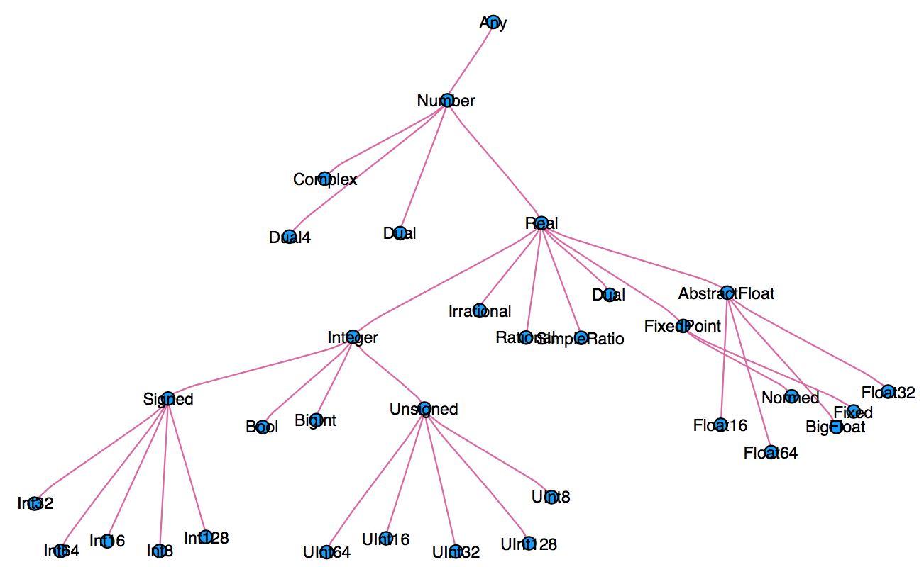
- You can explore type hierarchy with
typeof(),supertype(), andsubtypes().
typeof(1.0), typeof(1)
supertype(Float64)
subtypes(AbstractFloat)
# Is Float64 a subtype of AbstractFloat?
Float64 <: AbstractFloat
What properties does a
Numberhave?- You can add numbers (
+) - You can multiply numbers (
*) - etc.
- You can add numbers (
This definition is too broad, since some things can't be added
g(x) = x + x
This definition is too restrictive, since any Number can be added
g(x::Float64) = x + x
This will automatically work on the entire type tree above!
g(x::Number) = x + x
This is a lot nicer than
function g(x)
  if isa(x, Number)
      return x + x
  else
      throw(ArgumentError("x should be a number"))
  end
end
Just-in-time compilation (JIT)
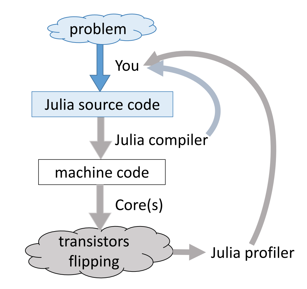
Following figures and some examples are taken from Arch D. Robinson's slides Introduction to Writing High Performance Julia.
 |
 |
|---|---|
x = randn(100)
@time sum(x) # first call invokes compilation
@time sum(x) # second run doesn't need compilation anymore
Julia's efficiency results from its capabilities to infer the types of all variables within a function and then call LLVM to generate optimized machine code at run-time.
g(x) = x + x
This function will work on any type which has a method for +.
@show g(2)
@show g(2.0);
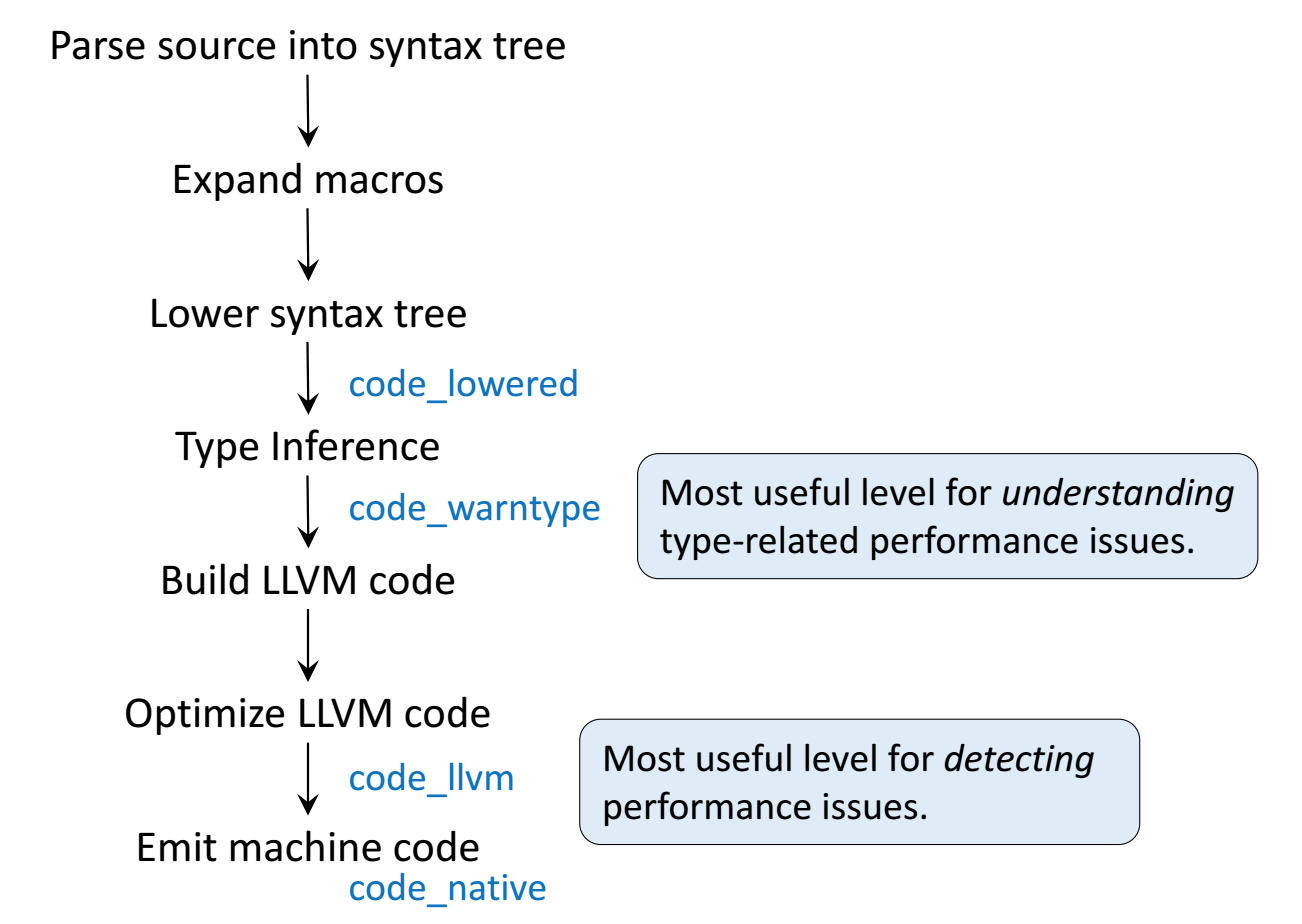
This the abstract syntax tree.
@code_lowered g(2)
Peek at the compiled code (LLVM bitcode) with @code_llvm
@code_llvm g(2)
@code_llvm g(2.0)
We didn't provide a type annotation. But different code gets called depending on the argument type!
In R or Python,
g(2)andg(2.0)would use the same code for both.In Julia,
g(2)andg(2.0)dispatches to optimized code forInt64andFloat64, respectively.For integer input
x, LLVM compiler is smart enough to knowx + xis simple shiftingxby 1 bit, which is faster than addition.
This is assembly code, which is machin dependent.
@code_native g(2)
@code_native g(2.0)
Profiling Julia code
Julia has several built-in tools for profiling. The @time marco outputs run time and heap allocation.
function tally(x)
    s = 0
    for v in x
        s += v
    end
    s
end

a = rand(10000)
@time tally(a) # warm up: include compile time
@time tally(a)
For more robust benchmarking, the BenchmarkTools.jl package is highly recommended.
using BenchmarkTools

@benchmark tally(a)
We see the heap allocation (average 10.73% GC) is suspiciously high.
The Profile module gives line by line profile results.
a = rand(10000000)
Profile.clear()
@profile tally(a)
Profile.print(format=:flat)
Memory profiling
Detailed memory profiling requires a detour. First let's write a script bar.jl, which contains the workload function tally and a wrapper for profiling.
;cat bar.jl
Next, in terminal, we run the script with --track-allocation=user option.
;julia --track-allocation=user bar.jl
The profiler outputs a file bar.jl.mem.
;cat bar.jl.mem
We see line 4 is allocating suspicious amount of heap memory.
Type stability
The key to writing performant Julia code is to be type stable, such that Julia is able to infer types of all variables and output of a function from the types of input arguments.
Is the tally function type stable? How to diagnose and fix it?
@code_warntype tally(rand(100))
In this case, Julia fails to infer the type of the reduction variable s, which has to be boxed in heap memory at run time.


What's the fix?
Plotting in Julia
The three most popular options (as far as I can tell) are
- Gadfly.jl
- Julia version of
ggplot2in R
- Julia version of
- PyPlot.jl
- Wrapper for Python's matplotlib
- Plots.jl (my personal favorite)
- Defines an unified interface for plotting
- maps arguments to different plotting "backends"
- PyPlot, GR, PlotlyJS, and many more
using Plots

x = randn(50, 2);
pyplot()  # set the backend to PyPlot
plot(x)

plotly()  # change backend to Plotly
plot(x)
gr()   # change backend to GR
plot(x)
gr()
@gif for i in 1:20
    plot(x -> sin(x) / (.2i), 0, i, xlim=(0, 20), ylim=(-.75, .75))
    scatter!(x -> cos(x) * .01 * i, 0, i, m=1)
end
# Nondeterministic algorithm for plotting functions
# Tries to do higher sampling where the function changes the most
scatter(sin, -3, 3)
plot!(sin)
x = randn()
p = plot([x])
@gif for i in 1:100
    x += randn()
    push!(p, x)
end
