Iterative Methods for Solving Linear Equations
Introduction
So far we have considered direct methods for solving linear equations.
- Direct methods (flops fixed a priori) vs iterative methods:
- Direct method (GE/LU, Cholesky, QR, SVD): good for dense, small or moderate sized $\mathbf{A}$
- Iterative methods (Jacobi, Gauss-Seidal, SOR, conjugate-gradient, GMRES): good for large, sparse, structured linear system, parallel computing, warm start
PageRank problem (HW3)
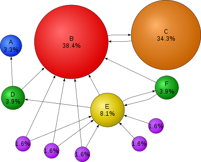
$\mathbf{A} \in \{0,1\}^{n \times n}$ the connectivity matrix of webpages with entries $$ \begin{eqnarray*} a_{ij} = \begin{cases} 1 & \text{if page $i$ links to page $j$} \\ 0 & \text{otherwise} \end{cases}. \end{eqnarray*} $$ $n \approx 10^9$ in May 2017.
$r_i = \sum_j a_{ij}$ is the out-degree of page $i$.
Larry Page imagines a random surfer wandering on internet according to following rules:
- From a page $i$ with $r_i>0$
- with probability $p$, (s)he randomly chooses a link on page $i$ (uniformly) and follows that link to the next page
- with probability $1-p$, (s)he randomly chooses one page from the set of all $n$ pages (uniformly) and proceeds to that page
- From a page $i$ with $r_i=0$ (a dangling page), (s)he randomly chooses one page from the set of all $n$ pages (uniformly) and proceeds to that page
- From a page $i$ with $r_i>0$
The process defines a Markov chain on the space of $n$ pages. Stationary distribution of this Markov chain gives the ranks (probabilities) of each page.
Stationary distribution is the top left eigenvector of the transition matrix $\mathbf{P}$ corresponding to eigenvalue 1. Equivalently it can be cast as a linear equation.
Gene Golub: Largest matrix computation in world.
GE/LU will take $2 \times (10^9)^3/3/10^{12} \approx 6.66 \times 10^{14}$ seconds $\approx 20$ million years on a tera-flop supercomputer!
Iterative methods come to the rescue.
Jacobi method

Solve $\mathbf{A} \mathbf{x} = \mathbf{b}$.
Jacobi iteration: $$ x_i^{(t+1)} = \frac{b_i - \sum_{j=1}^{i-1} a_{ij} x_j^{(t)} - \sum_{j=i+1}^n a_{ij} x_j^{(t)}}{a_{ii}}. $$
With splitting: $\mathbf{A} = \mathbf{L} + \mathbf{D} + \mathbf{U}$, Jacobi iteration can be written as $$ \mathbf{D} \mathbf{x}^{(t+1)} = - (\mathbf{L} + \mathbf{U}) \mathbf{x}^{(t)} + \mathbf{b}, $$ i.e., $$ \mathbf{x}^{(t+1)} = - \mathbf{D}^{-1} (\mathbf{L} + \mathbf{U}) \mathbf{x}^{(t)} + \mathbf{D}^{-1} \mathbf{b} = - \mathbf{D}^{-1} \mathbf{A} \mathbf{x}^{(t)} + \mathbf{x}^{(t)} + \mathbf{D}^{-1} \mathbf{b}. $$
One round costs $2n^2$ flops with an unstructured $\mathbf{A}$. Gain over GE/LU if converges in $o(n)$ iterations. Saving is huge for sparse or structured $\mathbf{A}$. By structured, we mean the matrix-vector multiplication $\mathbf{A} \mathbf{v}$ is fast ($O(n)$ or $O(n \log n)$).
Gauss-Seidel method

Gauss-Seidel (GS) iteration: $$ x_i^{(t+1)} = \frac{b_i - \sum_{j=1}^{i-1} a_{ij} x_j^{(t+1)} - \sum_{j=i+1}^n a_{ij} x_j^{(t)}}{a_{ii}}. $$
With splitting, $(\mathbf{D} + \mathbf{L}) \mathbf{x}^{(t+1)} = - \mathbf{U} \mathbf{x}^{(t)} + \mathbf{b}$, i.e., $$ \mathbf{x}^{(t+1)} = - (\mathbf{D} + \mathbf{L})^{-1} \mathbf{U} \mathbf{x}^{(t)} + (\mathbf{D} + \mathbf{L})^{-1} \mathbf{b}. $$
GS converges for any $\mathbf{x}^{(0)}$ for symmetric and pd $\mathbf{A}$.
Convergence rate of Gauss-Seidel is the spectral radius of the $(\mathbf{D} + \mathbf{L})^{-1} \mathbf{U}$.
Successive over-relaxation (SOR)
SOR: $$ x_i^{(t+1)} = \omega \left( b_i - \sum_{j=1}^{i-1} a_{ij} x_j^{(t+1)} - \sum_{j=i+1}^n a_{ij} x_j^{(t)} \right) / a_{ii} + (1-\omega) x_i^{(t)}, $$ i.e., $$ \mathbf{x}^{(t+1)} = (\mathbf{D} + \omega \mathbf{L})^{-1} [(1-\omega) \mathbf{D} - \omega \mathbf{U}] \mathbf{x}^{(t)} + (\mathbf{D} + \omega \mathbf{L})^{-1} (\mathbf{D} + \mathbf{L})^{-1} \omega \mathbf{b}. $$
Need to pick $\omega \in [0,1]$ beforehand, with the goal of improving convergence rate.
Conjugate gradient method
Conjugate gradient and its variants are the top-notch iterative methods for solving huge, structured linear systems.
Solving $\mathbf{A} \mathbf{x} = \mathbf{b}$ is equivalent to minimizing the quadratic function $\frac{1}{2} \mathbf{x}^T \mathbf{A} \mathbf{x} - \mathbf{b}^T \mathbf{x}$.
To do later, when we study optimization.
Kershaw's results for a fusion problem.
| Method | Number of Iterations |
|---|---|
| Gauss Seidel | 208,000 |
| Block SOR methods | 765 |
| Incomplete Cholesky conjugate gradient | 25 |
Numerical examples
The IterativeSolvers.jl package implements many commonly used iterative solvers.
using BenchmarkTools, IterativeSolvers

srand(280)

n = 4000
# a sparse pd matrix, about 0.5% non-zero entries
A = sprand(n, n, 0.002)
A = A + A' + (2n) * I
@show typeof(A)
b = randn(n)
Afull = full(A)
@show typeof(Afull)
# actual sparsity level
countnz(A) / length(A)
# dense matrix-vector multiplication
@benchmark Afull * b
# sparse matrix-vector multiplication
@benchmark A * b
# dense solve via Cholesky
xchol = cholfact(Afull) \ b
@benchmark cholfact(Afull) \ b
# Jacobi solution is fairly close to Cholesky solution
xjacobi, = jacobi(A, b)
@show vecnorm(xjacobi - xchol)
@benchmark jacobi(A, b)
# Gauss-Seidel solution is fairly close to Cholesky solution
xgs, = gauss_seidel(A, b)
vecnorm(xgs - xchol)
@benchmark gauss_seidel(A, b)
# symmetric SOR with ω=0.75
xsor, = ssor(A, b, 0.75)
vecnorm(xsor - xchol)
@benchmark sor(A, b, 0.75)
# conjugate gradient
xcg, = cg(A, b)
vecnorm(xcg - xchol)
@benchmark cg(A, b)