Eigen-decomposition and SVD
Our last topic on numerical linear algebra is eigen-decomposition and singular value decomposition (SVD). We already saw the wide applications of QR decomposition in least squares problem and solving square and under-determined linear equations. Eigen-decomposition and SVD can be deemed as more thorough orthogonalization of a matrix. We start with a brief review of the related linear algebra.
Linear algebra review: eigen-decomposition
Eigenvalues are defined as roots of the characteristic equation $\det(\lambda \mathbf{I}_n - \mathbf{A})=0$.
If $\lambda$ is an eigenvalue of $\mathbf{A}$, then there exist non-zero $\mathbf{x}, \mathbf{y} \in \mathbb{R}^n$ such that $\mathbf{A} \mathbf{x} = \lambda \mathbf{x}$ and $\mathbf{y}^T \mathbf{A} = \lambda \mathbf{y}^T$. $\mathbf{x}$ and $\mathbf{x}$ are called the (column) eigenvector and row eigenvector of $\mathbf{A}$ associated with the eigenvalue $\lambda$.
$\mathbf{A}$ is singular if and only if it has at least one 0 eigenvalue.
Eigenvectors associated with distinct eigenvalues are linearly independent.
Eigenvalues of an upper or lower triangular matrix are its diagonal entries: $\lambda_i = a_{ii}$.
Eigenvalues of an idempotent matrix are either 0 or 1.
Eigenvalues of an orthogonal matrix have complex modulus 1.
In most statistical applications, we deal with eigenvalues/eigenvectors of symmetric matrices. The eigenvalues and eigenvectors of a real symmetric matrix are real.
Eigenvectors associated with distinct eigenvalues of a symmetry matrix are orthogonal.
Eigen-decompostion of a symmetric matrix: $\mathbf{A} = \mathbf{U} \Lambda \mathbf{U}^T$, where
- $\Lambda = \text{diag}(\lambda_1,\ldots,\lambda_n)$
- columns of $\mathbf{U}$ are the eigenvectors, which are (or can be chosen to be) mutually orthonormal. Thus $\mathbf{U}$ is an orthogonal matrix.
A real symmetric matrix is positive semidefinite (positive definite) if and only if all eigenvalues are nonnegative (positive).
Spectral radius $\rho(\mathbf{A}) = \max_i |\lambda_i|$.
$\mathbf{A} \in \mathbb{R}^{n \times n}$ a square matrix (not required to be symmetric), then $\text{tr}(\mathbf{A}) = \sum_i \lambda_i$ and $\det(\mathbf{A}) = \prod_i \lambda_i$.
Linear algebra review: singular value decomposition (SVD)
Singular value decomposition (SVD): For a rectangular matrix $\mathbf{A} \in \mathbb{R}^{m \times n}$, let $p = \min\{m,n\}$, then we have the SVD $$ \mathbf{A} = \mathbf{U} \Sigma \mathbf{V}^T, $$ where
- $\mathbf{U} = (\mathbf{u}_1,\ldots,\mathbf{u}_m) \in \mathbb{R}^{m \times m}$ is orthogonal
- $\mathbf{V} = (\mathbf{v}_1,\ldots,\mathbf{v}_n) \in \mathbb{R}^{n \times n}$ is orthogonal
- $\Sigma = \text{diag}(\sigma_1, \ldots, \sigma_p) \in \mathbb{R}^{m \times n}$, $\sigma_1 \ge \sigma_2 \ge \cdots \ge \sigma_p \ge 0$.
$\sigma_i$ are called the singular values, $\mathbf{u}_i$ are the left singular vectors, and $\mathbf{v}_i$ are the right singular vectors.
Thin/Skinny SVD. Assume $m \ge n$. $\mathbf{A}$ can be factored as $$ \mathbf{A} = \mathbf{U}_n \Sigma_n \mathbf{V}^T = \sum_{i=1}^n \sigma_i \mathbf{u}_i \mathbf{v}_i^T, $$ where
- $\mathbf{U}_n \in \mathbb{R}^{m \times n}$, $\mathbf{U}_n^T \mathbf{U}_n = \mathbf{I}_n$
- $\mathbf{V} \in \mathbb{R}^{n \times n}$, $\mathbf{V}^T \mathbf{V} = \mathbf{I}_n$
- $\Sigma_n = \text{diag}(\sigma_1,\ldots,\sigma_n) \in \mathbb{R}^{n \times n}$, $\sigma_1 \ge \sigma_2 \ge \cdots \ge \sigma_n \ge 0$
Denote $\sigma(\mathbf{A})=(\sigma_1,\ldots,\sigma_p)^T$. Then
- $r = \text{rank}(\mathbf{A}) = \# \text{ nonzero singular values} = \|\sigma(\mathbf{A})\|_0$
- $\mathbf{A} = \mathbf{U}_r \Sigma_r \mathbf{V}_r^T = \sum_{i=1}^r \sigma_i \mathbf{u}_i \mathbf{v}_i^T$
- $\|\mathbf{A}\|_{\text{F}} = (\sum_{i=1}^p \sigma_i^2)^{1/2} = \|\sigma(\mathbf{A})\|_2$
- $\|\mathbf{A}\|_2 = \sigma_1 = \|\sigma(\mathbf{A})\|_\infty$
Assume $\text{rank}(\mathbf{A}) = r$ and partition $$ \begin{eqnarray*} \mathbf{U} &=& (\mathbf{U}_r, \tilde{\mathbf{U}}_r) \in \mathbb{R}^{m \times m} \\ \mathbf{V} &=& (\mathbf{V}_r, \tilde{\mathbf{V}}_r) \in \mathbb{R}^{n \times n}. \end{eqnarray*} $$ Then
- ${\cal C}(\mathbf{A}) = {\cal C}(\mathbf{U}_r)$, ${\cal N}(\mathbf{A}^T) = {\cal C}(\tilde{\mathbf{U}}_r)$
- ${\cal N}(\mathbf{A}) = {\cal C}(\tilde{\mathbf{V}}_r)$, ${\cal C}(\mathbf{A}^T) = {\cal C}(\mathbf{V}_r)$
- $\mathbf{U}_r \mathbf{U}_r^T$ is the orthogonal projection onto ${\cal C}(\mathbf{A})$
- $\tilde{\mathbf{U}}_r \tilde{\mathbf{U}}_r^T$ is the orthogonal projection onto ${\cal N}(\mathbf{A}^T)$
- $\mathbf{V}_r \mathbf{V}_r^T$ is the orthogonal projection onto ${\cal C}(\mathbf{A}^T)$
- $\tilde{\mathbf{V}}_r \tilde{\mathbf{V}}_r^T$ is the orthogonal projection onto ${\cal N}(\mathbf{A})$
Relation to eigen-decomposition. Using thin SVD, $$ \begin{eqnarray*} \mathbf{A}^T \mathbf{A} &=& \mathbf{V} \Sigma \mathbf{U}^T \mathbf{U} \Sigma \mathbf{V}^T = \mathbf{V} \Sigma^2 \mathbf{V}^T \\ \mathbf{A} \mathbf{A}^T &=& \mathbf{U} \Sigma \mathbf{V}^T \mathbf{V} \Sigma \mathbf{U}^T = \mathbf{U} \Sigma^2 \mathbf{U}^T. \end{eqnarray*} $$ In principle we can obtain singular triplets of $\mathbf{A}$ by doing two eigen-decompositions.
Another relation to eigen-decomposition. Using thin SVD, $$ \begin{eqnarray*} \begin{pmatrix} \mathbf{0}_{n \times n} & \mathbf{A}^T \\ \mathbf{A} & \mathbf{0}_{m \times m} \end{pmatrix} = \frac{1}{\sqrt 2} \begin{pmatrix} \mathbf{V} & \mathbf{V} \\ \mathbf{U} & -\mathbf{U} \end{pmatrix} \begin{pmatrix} \Sigma & \mathbf{0}_{n \times n} \\ \mathbf{0}_{n \times n} & - \Sigma \end{pmatrix} \frac{1}{\sqrt 2} \begin{pmatrix} \mathbf{V}^T & \mathbf{U}^T \\ \mathbf{V}^T & - \mathbf{U}^T \end{pmatrix}. \end{eqnarray*} $$ Hence any symmetric eigen-solver can produce the SVD of a matrix $\mathbf{A}$ without forming $\mathbf{A} \mathbf{A}^T$ or $\mathbf{A}^T \mathbf{A}$.
Yet another relation to eigen-decomposition: If the eigen-decomposition of a real symmetric matrix is $\mathbf{A} = \mathbf{W} \Lambda \mathbf{W}^T = \mathbf{W} \text{diag}(\lambda_1, \ldots, \lambda_n) \mathbf{W}^T$, then $$ \begin{eqnarray*} \mathbf{A} = \mathbf{W} \Lambda \mathbf{W}^T = \mathbf{W} \begin{pmatrix} |\lambda_1| & & \\ & \ddots & \\ & & |\lambda_n| \end{pmatrix} \begin{pmatrix} \text{sgn}(\lambda_1) & & \\ & \ddots & \\ & & \text{sgn}(\lambda_n) \end{pmatrix} \mathbf{W}^T \end{eqnarray*} $$ is the SVD of $\mathbf{A}$.
Applications of eigen-decomposition and SVD
Principal components analysis (PCA).
$\mathbf{X} \in \mathbb{R}^{n \times p}$ is a centered data matrix. Perform SVD $\mathbf{X} = \mathbf{U} \Sigma \mathbf{V}^T$ or equivalently $\mathbf{X}^T \mathbf{X} = \mathbf{V} \Sigma^2 \mathbf{V}^T$. The linear combinations $\tilde{\mathbf{x}}_i = \mathbf{X} \mathbf{v}_i$ are the principal components (PC) and have variance $\sigma_i^2$.
- Dimension reduction: reduce dimensionality $p$ to $q \ll p$. Use top PCs $\tilde{\mathbf{x}}_1, \ldots, \tilde{\mathbf{x}}_q$ in visualization and downstream analysis.

Above picture is from the article Genes mirror geography within Europe by Novembre et al (2008) published in Nature.
- Use PCs to adjust for confounding - a serious issue in association studies in large data sets.
- Use of PCA to adjust for confounding in modern genetic studies is proposed in the paper Principal components analysis corrects for stratification in genome-wide association studies by Price et al (2006) published in Nature Genetics. It has been cited 5,312 times as of May 8, 2017.
Low rank approximation
For example, image/data compression. Find a low rank approximation of data matrix $\mathbf{x}$.
Eckart-Young theorem:
$$
\min_{\text{rank}(\mathbf{Y})=r} \|\mathbf{X} - \mathbf{Y} \|_{\text{F}}^2
$$
is achieved by $\mathbf{Y} = \sum_{i=1}^r \sigma_i \mathbf{u}_i \mathbf{v}_i^T$ with optimal value $\sum_{i=r}^{p} \sigma_i^2$, where $(\sigma_i, \mathbf{u}_i, \mathbf{v}_i)$ are singular values and vectors of $\mathbf{X}$.
- Gene Golub's $897 \times 598$ picture requires $2691 \times 598 \times 8 = 12,873,744$ bytes (3 RGB channels).
- Rank 120 approximation requires $120 \times (2691+598) \times 8 = 3,157,440$ bytes.
- Rank 50 approximation requires $50 \times (2691+598) \times 6 = 1,315,600$ bytes.
- Rank 12 approximation requires $12 \times (2691+598) \times 6 = 315,744$ bytes.


Moore-Penrose (MP) inverse
Using thin SVD,
$$
\mathbf{A}^+ = \mathbf{V} \Sigma^+ \mathbf{U}^T,
$$
where $\Sigma^+ = \text{diag}(\sigma_1^{-1}, \ldots, \sigma_r^{-1}, 0, \ldots, 0)$, $r= \text{rank}(\mathbf{A})$. This is how the pinv function is implemented in Julia.
X = randn(5, 3)
pinv(X)
@which pinv(X)
Least squares
Given thin SVD $\mathbf{X} = \mathbf{U} \Sigma \mathbf{V}^T$, $$ \begin{eqnarray*} \widehat \beta &=& (\mathbf{X}^T \mathbf{X})^- \mathbf{X}^T \mathbf{y} \\ &=& (\mathbf{V} \Sigma^2 \mathbf{V}^T)^+ \mathbf{V} \Sigma \mathbf{U}^T \mathbf{y} \\ &=& \mathbf{V} (\Sigma^{2})^+ \mathbf{V}^T \mathbf{V} \Sigma \mathbf{U}^T \mathbf{y} \\ &=& \mathbf{V}_r \Sigma_r^{-1} \mathbf{U}_r^T \mathbf{y} \\ &=& \sum_{i=1}^r \left( \frac{\mathbf{u}_i^T \mathbf{y}}{\sigma_i} \right) \mathbf{v}_i \end{eqnarray*} $$ and $$ \begin{eqnarray*} \widehat{\mathbf{y}} &=& \mathbf{X} \widehat \beta = \mathbf{U}_r \mathbf{U}_r^T \mathbf{y}. \end{eqnarray*} $$ In general, SVD is more expensive than other approaches (Cholesky, Sweep, QR) we learnt. In some applications, SVD is computed for other purposes then we get least squares solution for free.
Ridge regression
In ridge regression, we minimize $$ \|\mathbf{y} - \mathbf{X} \beta\|_2^2 + \lambda \|\beta\|_2^2, $$ where $\lambda$ is a tuning parameter.
Ridge regression by augmented linear regression. Ridge regression problem is equivalent to $$ \left\| \begin{pmatrix} \mathbf{y} \\ \mathbf{0}_p \end{pmatrix} - \begin{pmatrix} \mathbf{X} \\ \sqrt \lambda \mathbf{I}_p \end{pmatrix} \beta \right\|_2^2. $$ Therefore any methods for linear regression can be applied.
Ridge regression by method of normal equation. The normal equation for the ridge problem is $$ (\mathbf{X}^T \mathbf{X} + \lambda \mathbf{I}_p) \beta = \mathbf{X}^T \mathbf{y}. $$ Therefore Cholesky or sweep operator can be used.
Ridge regression by SVD. If we obtain the (thin) SVD of $\mathbf{X}$ $$ \mathbf{X} = \mathbf{U} \Sigma_{p \times p} \mathbf{V}^T. $$ Then the normal equation reads $$ (\Sigma^2 + \lambda \mathbf{I}_p) \mathbf{V}^T \beta = \Sigma \mathbf{U}^T \mathbf{y} $$ and we get $$ \widehat \beta (\lambda) = \sum_{i=1}^p \frac{\sigma_i \mathbf{u}_i^T \mathbf{y}}{\sigma_i^2 + \lambda} \mathbf{v}_i = \sum_{i=1}^r \frac{\sigma_i \mathbf{u}_i^T \mathbf{y}}{\sigma_i^2 + \lambda} \mathbf{v}_i, \quad r = \text{rank}(\mathbf{X}). $$ It is clear that $$ \begin{eqnarray*} \lim_{\lambda \to 0} \widehat \beta (\lambda) = \widehat \beta_{\text{OLS}} \end{eqnarray*} $$ and $\|\widehat \beta (\lambda)\|_2$ is monotone decreasing as $\lambda$ increases.
Only one SVD is needed for all $\lambda$ (!), in contrast to the method of augmented linear regression, Cholesky, or sweep.
Other applications
See Chapters 8-9 of Numerical Analysis for Statisticians by Kenneth Lange (2010) for more applications of eigen-decomposition and SVD.
Algorithms for eigen-decomposition
One eigen-pair: power method
Power method iterates according to $$ \begin{eqnarray*} \mathbf{x}^{(t)} &\gets& \frac{1}{\|\mathbf{A} \mathbf{x}^{(t-1)}\|_2} \mathbf{A} \mathbf{x}^{(t-1)} \end{eqnarray*} $$ from an initial guess $\mathbf{x}^{(0)}$ of unit norm.
Suppose we arrange $|\lambda_1| > |\lambda_2| \ge \cdots \ge |\lambda_n|$ (the first inequality strict) with corresponding eigenvectors $\mathbf{u}_i$, and expand $\mathbf{x}^{(0)} = c_1 \mathbf{u}_1 + \cdots + c_n \mathbf{u}_n$, then $$ \begin{eqnarray*} \mathbf{x}^{(t)} &=& \frac{\left( \sum_i \lambda_i^t \mathbf{u}_i \mathbf{u}_i^T \right) \left( \sum_i c_i \mathbf{u}_i \right)}{\|\left( \sum_i \lambda_i^t \mathbf{u}_i \mathbf{u}_i^T \right) \left( \sum_i c_i \mathbf{u}_i \right)\|_2} \\ &=& \frac{\sum_i c_i \lambda_i^t \mathbf{u}_i}{\|\sum_i c_i \lambda_i^t \mathbf{u}_i\|_2} \\ &=& \frac{c_1 \mathbf{u}_1 + c_2 (\lambda_2/\lambda_1)^t \mathbf{u}_2 + \cdots + c_n (\lambda_n/\lambda_1)^t \mathbf{u}_n}{\|c_1 \mathbf{u}_1 + c_2 (\lambda_2/\lambda_1)^t \mathbf{u}_2 + \cdots + c_n (\lambda_n/\lambda_1)^t \mathbf{u}_n\|_2} \left( \frac{\lambda_1}{|\lambda_1|} \right)^t. \end{eqnarray*} $$ Thus $\mathbf{x}^{(t)} - \frac{c_1 \mathbf{u}_1}{\|c_1 \mathbf{u}_1\|_2} \left( \frac{\lambda_1}{|\lambda_1|} \right)^t \to 0$ as $t \to \infty$. The convergence rate is $|\lambda_2|/|\lambda_1|$.
$\lambda_1^{(t)} = \mathbf{x}^{(t)T} \mathbf{A} \mathbf{x}^{(t)}$ converges to $\lambda_1$.
Inverse power method for finding the eigenvalue of smallest absolute value: Substitute $\mathbf{A}$ by $\mathbf{A}^{-1}$ in the power method. (E.g., pre-compute LU or Cholesky of $\mathbf{A}$).
Shifted inverse power: Substitute $(\mathbf{A} - \mu \mathbf{I})^{-1}$ in the power method. It converges to an eigenvalue close to the given $\mu$.
Rayleigh quotient iteration: Substitute $(\mathbf{A} - \mu^{(t-1)} \mathbf{I})^{-1}$, where $\mu^{(t-1)} = \mathbf{x}^{(t-1)T} \mathbf{A} \mathbf{x}^{(t-1)}$ in the shifted inverse method. Faster convergence.
Example: PageRank problem seeks top left eigenvector of transition matrix $\mathbf{P}$ and costs $O(n)$ per iteration.
Top $r$ eigen-pairs: orthogonal iteration
Generalization of power method to higher dimensional invariant subspace.
Orthogonal iteration: Initialize $\mathbf{Q}^{(0)} \in \mathbb{R}^{n \times r}$ with orthonormal columns. For $t=1,2,\ldots$, $$ \begin{eqnarray*} \mathbf{Z}^{(t)} &\gets& \mathbf{A} \mathbf{Q}^{(t-1)} \quad \text{($2n^2r$ flops)} \\ \mathbf{Q}^{(t)} \mathbf{R}^{(t)} &\gets& \mathbf{Z}^{(t)} \quad \text{(QR factorization)}%, $nr^2 - r^3/3$ flops)} \end{eqnarray*} $$
$\mathbf{Z}^{(t)}$ converges to the eigenspace of the largest $r$ eigenvalues if they are real and separated from remaining spectrum. The convergence rate is $|\lambda_{r+1}|/|\lambda_r|$.
(Impractical) full eigen-decomposition: QR iteration
Assume $\mathbf{A} \in \mathbb{R}^{n \times n}$ symmetric.
Take $r=n$ in the orthogonal iteration. Then $\mathbf{Q}^{(t)}$ converges to the eigenspace $\mathbf{U}$ of $\mathbf{A}$. This implies that $$ \mathbf{T}^{(t)} := \mathbf{Q}^{(t)T} \mathbf{A} \mathbf{Q}^{(t)} $$ converges to a diagonal form $\Lambda = \text{diag}(\lambda_1, \ldots, \lambda_n)$.
Note how to compute $\mathbf{T}^{(t)}$ from $\mathbf{T}^{(t-1)}$ $$ \begin{eqnarray*} \mathbf{T}^{(t-1)} &=& \mathbf{Q}^{(t-1)T} \mathbf{A} \mathbf{Q}^{(t-1)} = \mathbf{Q}^{(t-1)T} (\mathbf{A} \mathbf{Q}^{(t-1)}) = (\mathbf{Q}^{(t-1)T} \mathbf{Q}^{(t)}) \mathbf{R}^{(t)} \\\mathbf{A} \mathbf{T}^{(t)} &=& \mathbf{Q}^{(t)T} \mathbf{A} \mathbf{Q}^{(t)} = \mathbf{Q}^{(t)T} \mathbf{A} \mathbf{Q}^{(t-1)} \mathbf{Q}^{(t-1)T} \mathbf{Q}^{(t)} = \mathbf{R}^{(t)} ( \mathbf{Q}^{(t-1)T} \mathbf{Q}^{(t)}). \end{eqnarray*} $$
QR iteration: Initialize $\mathbf{U}^{(0)} \in \mathbb{R}^{n \times n}$ orthogonal and set $\mathbf{T}^{(0)} = \mathbf{U}^{(0)T} \mathbf{A} \mathbf{U}^{(0)}$. \ For $t=1,2,\ldots$ $$ \begin{eqnarray*} \mathbf{U}^{(t)} \mathbf{R}^{(t)} &\gets& \mathbf{T}^{(t-1)} \quad \text{(QR factorization)} \\ \mathbf{T}^{(t)} &\gets& \mathbf{R}^{(t)} \mathbf{U}^{(t)} \end{eqnarray*} $$
QR iteration is expensive in general: $O(n^3)$ per iteration and linear convergence rate.
QR algorithm for symmetric eigen-decomposition
Assume $\mathbf{A} \in \mathbb{R}^{n \times n}$ symmetric.
Reading: The QR algorithm by Beresford N. Parlett.
This is the algorithm implemented in LAPACK: used by Julia, Matlab, R.
Idea: Tri-diagonalization (by Householder) + QR iteration on the tri-diagonal system with implicit shift.
Step 1: Householder tri-diagonalization: $4n^3/3$ for eigenvalues only, $8n^3/3$ for both eigenvalues and eigenvectors. (Why can't we apply Householder to make it diagonal directly?)
Step 2: QR iteration on the tridiagonal matrix. Implicit shift accelerates convergence rate. On average 1.3-1.6 QR iteration per eigenvalue, $\sim 20n$ flops per QR iteration. So total operation count is about $30n^2$. Eigenvectors need an extra of about $6n^3$ flops.
| Eigenvalue | Eigenvector | |
|---|---|---|
| Householder reduction | $4n^3/3$ | $4n^3/3$ |
| QR with implicit shift | $\sim 30n^2$ | $\sim 6n^3$ |
Message: Don't request eigenvectors unless necessary. Use
eigvalsin Julia to request only eigenvalues.The unsymmetric QR algorithm obtains the real Schur decomposition of an asymmetric matrix $\mathbf{A}$.
srand(280)
A = Symmetric(randn(5, 5), :U)

Aeig = eigfact(A)
@which eigfact(A)
# eigen-values
Aeig[:values]
# eigen-vectors
Aeig[:vectors]
# inversion by eigen-decomposition
inv(Aeig)
@which inv(Aeig)
# determinant by eigen-decomposition
det(Aeig)
@which det(Aeig)
@which eigvals(A)
@which eigmax(A)
@which eigmin(A)
Don't request eigenvectors unless needed.
using BenchmarkTools

srand(280)

n = 1000
A = Symmetric(randn(n, n), :U)
@benchmark eigvals(A)
@benchmark eigfact(A)
Algorithm for singular value decomposition (SVD)

Assume $\mathbf{A} \in \mathbb{R}^{m \times n}$ and we seek the SVD $\mathbf{A} = \mathbf{U} \mathbf{D} \mathbf{V}^T$.
Golub-Kahan-Reinsch algorithm:
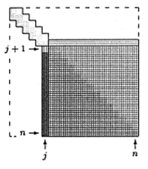
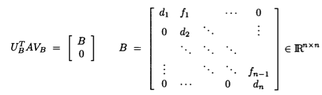
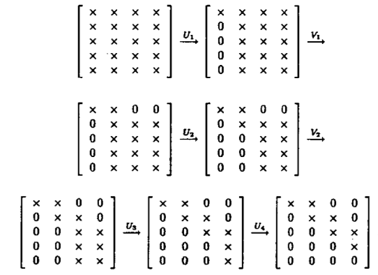
- Stage 1: Transform $\mathbf{A}$ to an upper bidiagonal form $\mathbf{B}$ (by Householder).
- Stage 2: Apply implicit-shift QR iteration to the tridiagonal matrix $\mathbf{B}^T \mathbf{B}$ implicitly.
See Section 8.6 of Matrix Computation by Gene Golub and Charles Van Loan (2013) for more details.
$4m^2 n + 8mn^2 + 9n^3$ flops for a tall $(m \ge n)$ matrix.
Example
srand(280)

A = randn(5, 3)
Asvd = svdfact(A)
Asvd[:U]
# Vt is cheaper to extract than V
Asvd[:Vt]
Asvd[:V]
Asvd[:S]
Don't request singular vectors unless needed.
srand(280)

n, p = 1000, 500
A = randn(n, p)

@benchmark svdvals(A)
@benchmark svdfact(A)
Lanczos/Arnoldi iterative method for top eigen-pairs
Consider the Google PageRank problem. We want to find the top left eigenvector of the transition matrix $\mathbf{P}$. Direct methods such as (unsymmetric) QR or SVD takes forever. Iterative methods such as power method is feasible. However power method may take a large number of iterations.
Krylov subspace methods are the state-of-art iterative methods for obtaining the top eigen-values/vectors or singular values/vectors of large sparse or structured matrices.
Lanczos method: top eigen-pairs of a large symmetric matrix.
Arnoldi method: top eigen-pairs of a large asymmetric matrix.
Both methods are also adapted to obtain top singular values/vectors of large sparse or structured matrices.
We will give an overview of these methods together with the conjugate gradient method for solving large linear system.
eigsandsvdsin Julia and Matlab are wrappers of the ARPACK package, which implements Lanczos and Arnoldi methods.
using BenchmarkTools

srand(280)

n = 4000
# a sparse pd matrix, about 0.5% non-zero entries
A = sprand(n, n, 0.002)
A = A + A' + (2n) * I
@show typeof(A)
b = randn(n)
Afull = Symmetric(full(A))
@show typeof(Afull)
# actual sparsity level
countnz(A) / length(A)
# top 5 eigenvalues by LAPACK (QR algorithm)
eigvals(Afull, (n-4):n)
# top 5 eigenvalues by iterative methods
eigs(A; nev = 5, ritzvec = false)
@benchmark eigvals(Afull, (n-4):n)
@benchmark eigs(A; nev = 5, ritzvec = false)
@which eigs(A)
Jacobi method for symmetric eigen-decomposition
Assume $\mathbf{A} \in \mathbf{R}^{n \times n}$ is symmetric and we seek the eigen-decomposition $\mathbf{A} = \mathbf{U} \Lambda \mathbf{U}^T$.
Idea: Systematically reduce off-diagonal entries $$ \text{off}(\mathbf{A}) = \sum_i \sum_{j \ne i} a_{ij}^2 $$ by Jacobi rotations.
Jacobi/Givens rotations: $$ \begin{eqnarray*} \mathbf{J}(p,q,\theta) = \begin{pmatrix} 1 & & 0 & & 0 & & 0 \\ \vdots & \ddots & \vdots & & \vdots & & \vdots \\ 0 & & \cos(\theta) & & \sin(\theta) & & 0 \\ \vdots & & \vdots & \ddots & \vdots & & \vdots \\ 0 & & - \sin(\theta) & & \cos(\theta) & & 0 \\ \vdots & & \vdots & & \vdots & \ddots & \vdots \\ 0 & & 0 & & 0 & & 1 \end{pmatrix}, \end{eqnarray*} $$ $\mathbf{J}(p,q,\theta)$ is orthogonal.
Consider $\mathbf{B} = \mathbf{J}^T \mathbf{A} \mathbf{J}$. $\mathbf{B}$ preserves the symmetry and eigenvalues of $\mathbf{A}$. Taking $$ \begin{eqnarray*} \begin{cases} \tan (2\theta) = 2a_{pq}/({a_{qq}-a_{pp}}) & \text{if } a_{pp} \ne a_{qq} \\ \theta = \pi/4 & \text{if } a_{pp}=a_{qq} \end{cases} \end{eqnarray*} $$ forces $b_{pq}=0$.
Since orthogonal transform preserves Frobenius norm, we have $$ b_{pp}^2 + b_{qq}^2 = a_{pp}^2 + a_{qq}^2 + 2a_{pq}^2. $$ (Just check the 2-by-2 block)
Since $\|\mathbf{A}\|_{\text{F}} = \|\mathbf{B}\|_{\text{F}}$, this implies that the off-diagonal part $$ \text{off}(\mathbf{B}) = \text{off}(\mathbf{A}) - 2a_{pq}^2 $$ is decreased whenever $a_{pq} \ne 0$.
One Jacobi rotation costs $O(n)$ flops.
Classical Jacobi: search for the largest $|a_{ij}|$ at each iteration. $O(n^2)$ efforts!
$\text{off}(\mathbf{A}) \le n(n-1) a_{ij}^2$ and $\text{off}(\mathbf{B}) = \text{off}(\mathbf{A}) - 2 a_{ij}^2$ together implies $$ \text{off}(\mathbf{B}) \le \left( 1 - \frac{2}{n(n-1)} \right) \text{off}(\mathbf{A}). $$ Thus Jacobi method converges in $O(n^2)$ iterations.
In practice, cyclic-by-row implementation, to avoid the costly $O(n^2)$ search in the classical Jacobi.
Jacobi method attracts a lot recent attention because of its rich inherent parallelism.
Parallel Jacobi: ``merry-go-round" to generate parallel ordering.