MM Algorithm (KL Chapter 12)

- Recall our picture for understanding the ascent property of EM
EM as a minorization-maximization (MM) algorithm
- The $Q$ function constitutes a minorizing function of the objective function up to an additive constant $$ \begin{eqnarray*} L(\theta) &\ge& Q(\theta|\theta^{(t)}) + c^{(t)} \quad \text{for all } \theta \\ L(\theta^{(t)}) &=& Q(\theta^{(t)}|\theta^{(t)}) + c^{(t)} \end{eqnarray*} $$
- Maximizing the $Q$ function generates an ascent iterate $\theta^{(t+1)}$
Questions:
- Is EM principle only limited to maximizing likelihood model?
- Can we flip the picture and apply same principle to minimization problem?
- Is there any other way to produce such surrogate function?
These thoughts lead to a powerful tool - MM algorithm.
Lange, K., Hunter, D. R., and Yang, I. (2000). Optimization transfer using surrogate objective functions. J. Comput. Graph. Statist., 9(1):1-59. With discussion, and a rejoinder by Hunter and Lange.For maximization of $f(\theta)$ - minorization-maximization (MM) algorithm
- Minorization step: Construct a surrogate function $g(\theta|\theta^{(t)})$ that satisfies $$ \begin{eqnarray*} f(\theta) &\ge& g(\theta|\theta^{(t)}) \quad \text{(dominance condition)} \\ f(\theta^{(t)}) &=& g(\theta^{(t)}|\theta^{(t)}) \quad \text{(tangent condition)}. \end{eqnarray*} $$
- Maximization step: $$ \theta^{(t+1)} = \text{argmax} \, g(\theta|\theta^{(t)}). $$
Ascent property of minorization-maximization algorithm $$ f(\theta^{(t)}) = g(\theta^{(t)}|\theta^{(t)}) \le g(\theta^{(t+1)}|\theta^{(t)}) \le f(\theta^{(t+1)}). $$
EM is a special case of minorization-maximization (MM) algorithm.
For minimization of $f(\theta)$ - majorization-minimization (MM) algorithm
- Majorization step: Construct a surrogate function $g(\theta|\theta^{(t)})$ that satisfies $$ \begin{eqnarray*} f(\theta) &\le& g(\theta|\theta^{(t)}) \quad \text{(dominance condition)} \\ f(\theta^{(t)}) &=& g(\theta^{(t)}|\theta^{(t)}) \quad \text{(tangent condition)}. \end{eqnarray*} $$
- Minimization step: $$ \theta^{(t+1)} = \text{argmin} \, g(\theta|\theta^{(t)}). $$
Similarly we have the descent property of majorization-minimization algorithm.
Same convergence theory as EM.
Rational of the MM principle for developing optimization algorithms
- Free the derivation from missing data structure.
- Avoid matrix inversion.
- Linearize an optimization problem.
- Deal gracefully with certain equality and inequality constraints.
- Turn a non-differentiable problem into a smooth problem.
- Separate the parameters of a problem (perfect for massive, fine-scale parallelization).
Generic methods for majorization and minorization - inequalities
- Jensen's (information) inequality - EM algorithms
- Supporting hyperplane property of a convex function
- The Cauchy-Schwartz inequality - multidimensional scaling
- Arithmetic-geometric mean inequality
- Quadratic upper bound principle - Bohning and Lindsay
- ...
Numerous examples in KL chapter 12, or take Kenneth Lange's optimization course BIOMATH 210.
History: the name MM algorithm originates from the discussion (by Xiaoli Meng) and rejoinder of the Lange, Hunter, Yang (2000) paper.
MM example: non-negative matrix factorization (NNMF)
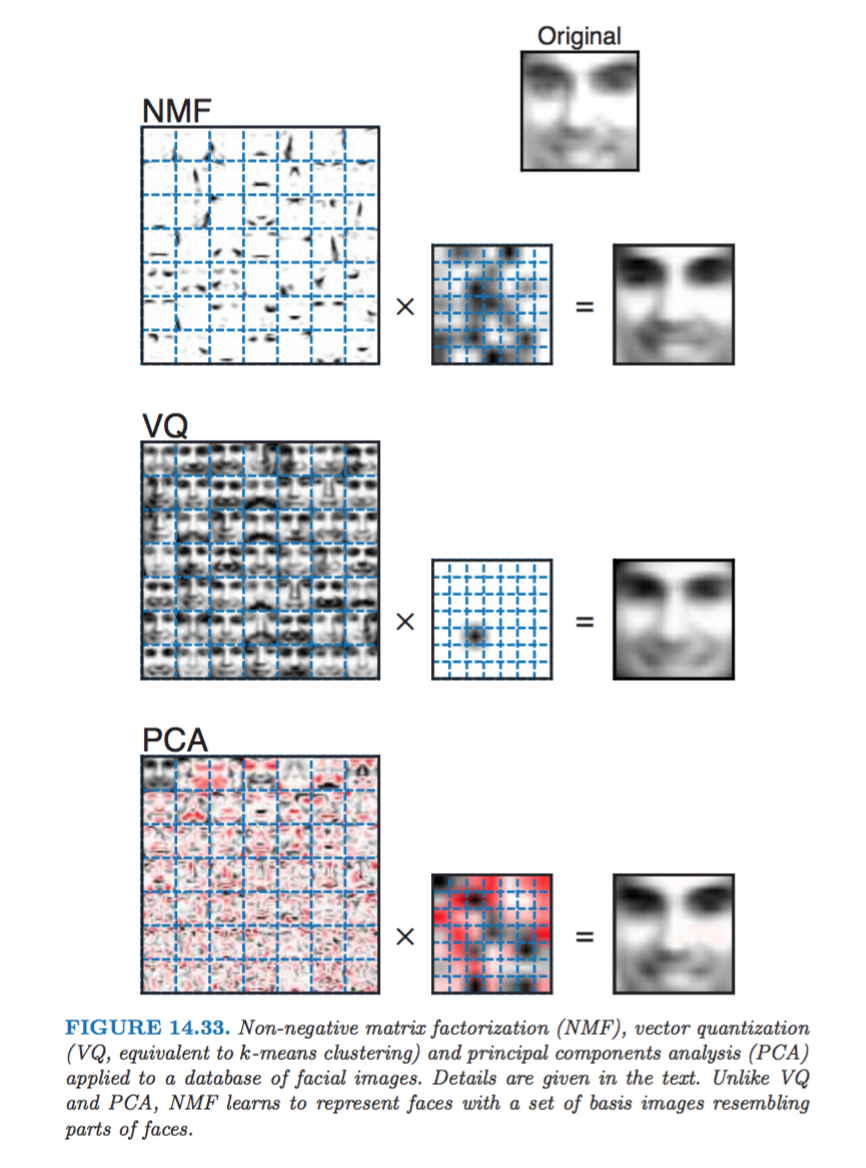
Nonnegative matrix factorization (NNMF) was introduced by Lee and Seung (1999, 2001) as an analog of principal components and vector quantization with applications in data compression and clustering.
In mathematical terms, one approximates a data matrix $\mathbf{X} \in \mathbb{R}^{m \times n}$ with nonnegative entries $x_{ij}$ by a product of two low-rank matrices $\mathbf{V} \in \mathbb{R}^{m \times r}$ and $\mathbf{W} \in \mathbb{R}^{r \times n}$ with nonnegative entries $v_{ik}$ and $w_{kj}$.
Consider minimization of the squared Frobenius norm $$ L(\mathbf{V}, \mathbf{W}) = \|\mathbf{X} - \mathbf{V} \mathbf{W}\|_{\text{F}}^2 = \sum_i \sum_j \left( x_{ij} - \sum_k v_{ik} w_{kj} \right)^2, \quad v_{ik} \ge 0, w_{kj} \ge 0, $$ which should lead to a good factorization.
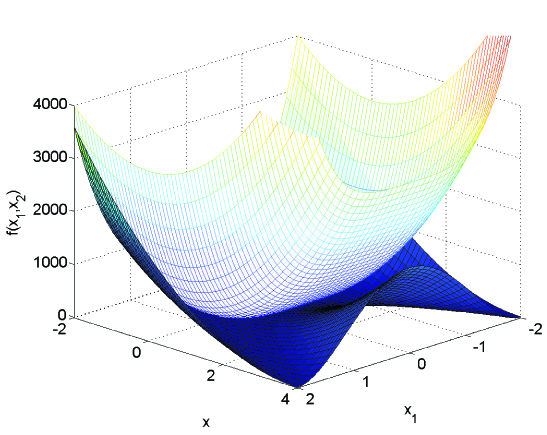
$L(\mathbf{V}, \mathbf{W})$ is not convex, but bi-convex. The strategy is to alternately update $\mathbf{V}$ and $\mathbf{W}$.
The key is the majorization, via convexity of the function $(x_{ij} - x)^2$, $$ \left( x_{ij} - \sum_k v_{ik} w_{kj} \right)^2 \le \sum_k \frac{a_{ikj}^{(t)}}{b_{ij}^{(t)}} \left( x_{ij} - \frac{b_{ij}^{(t)}}{a_{ikj}^{(t)}} v_{ik} w_{kj} \right)^2, $$ where $$ a_{ikj}^{(t)} = v_{ik}^{(t)} w_{kj}^{(t)}, \quad b_{ij}^{(t)} = \sum_k v_{ik}^{(t)} w_{kj}^{(t)}. $$
This suggests the alternating multiplicative updates $$ \begin{eqnarray*} v_{ik}^{(t+1)} &=& v_{ik}^{(t)} \frac{\sum_j x_{ij} w_{kj}^{(t)}}{\sum_j b_{ij}^{(t)} w_{kj}^{(t)}} \\ b_{ij}^{(t+1/2)} &=& \sum_k v_{ik}^{(t+1)} w_{kj}^{(t)} \\ w_{kj}^{(t+1)} &=& w_{kj}^{(t)} \frac{\sum_i x_{ij} v_{ik}^{(t+1)}}{\sum_i b_{ij}^{(t+1/2)} v_{ik}^{(t+1)}}. \end{eqnarray*} $$
The update is extremely simple $$ \begin{eqnarray*} \mathbf{B}^{(t)} &=& \mathbf{V}^{(t)} \mathbf{W}^{(t)} \\ \mathbf{V}^{(t+1)} &=& \mathbf{V}^{(t)} \odot (\mathbf{X} \mathbf{W}^{(t)T}) \oslash (\mathbf{B}^{(t)} \mathbf{W}^{(t)T}) \\ \mathbf{B}^{(t+1/2)} &=& \mathbf{V}^{(t+1)} \mathbf{W}^{(t)} \\ \mathbf{W}^{(t+1)} &=& \mathbf{W}^{(t)} \odot (\mathbf{X}^T \mathbf{V}^{(t+1)}) \oslash (\mathbf{B}^{(t+1/2)T} \mathbf{V}^{(t)}), \end{eqnarray*} $$ where $\odot$ denotes elementwise multiplication and $\oslash$ denotes elementwise division. If we start with $v_{ik}, w_{kj} > 0$, parameter iterates stay positive.
Monotoniciy of the algorithm is free (from MM principle).
Database #1 from the MIT Center for Biological and Computational Learning (CBCL, http://cbcl.mit.edu) reduces to a matrix X containing $m = 2,429$ gray-scale face images with $n = 19 \times 19 = 361$ pixels per face. Each image (row) is scaled to have mean and standard deviation 0.25.
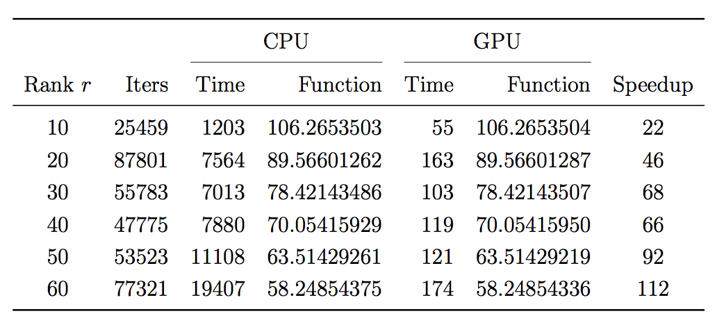
My implementation in around 2010:
CPU: Intel Core 2 @ 3.2GHZ (4 cores), implemented using BLAS in the GNU Scientific Library (GSL)
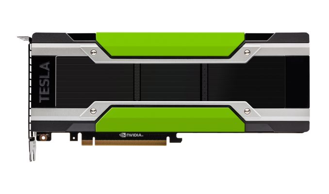
GPU: NVIDIA GeForce GTX 280 (240 cores), implemented using cuBLAS.
GPU
GPUs are ubiquitous: servers, desktops, and laptops.
Many EM/MM algorithms are particularly suitable for general purpose GPU (GPGPU) computing.
H Zhou, K Lange, and M Suchard. (2010) Graphics processing units and high-dimensional optimization, Statistical Science, 25:311-324.
GPGPU propels recent surgence of deep learning.
Following are typical computer systems in 2015.
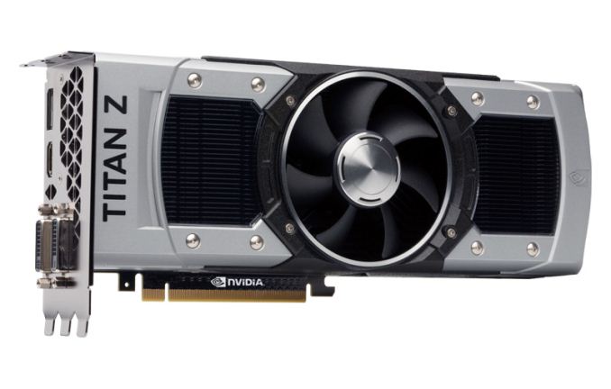
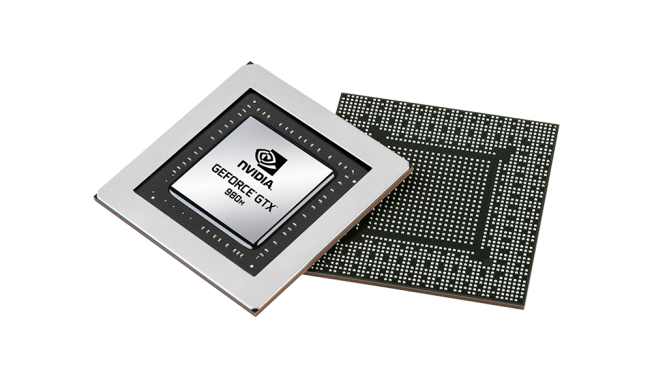
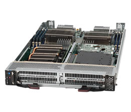
| NVIDIA GPUs | Tesla M40 | GTX Titan | GTX 980M |
|---|---|---|---|
 |
 |
 |
|
| Computers | servers, cluster | desktop | laptop |
 |
 |
 |
|
| Main usage | scientific computing | daily work, gaming | daily work |
| Memory | 12GB | 6GB | 1GB |
| Memory bandwidth | 288GB/sec | 288GB/sec | 160GB/sec |
| Number of cores | 3072 | 2688 | 1536 |
| Processor clock | 1.3GHz | 0.837GHz | 1.038GHz |
| Peak DP performance | 213Gflops | ||
| Peak SP performance | 6.84Tflops | 4.5Tflops | 3.189Tflops |
| Release price | \$4000 | \$999 | OEM |
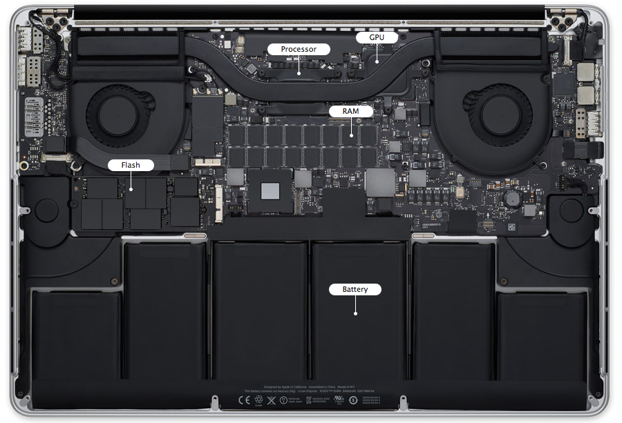
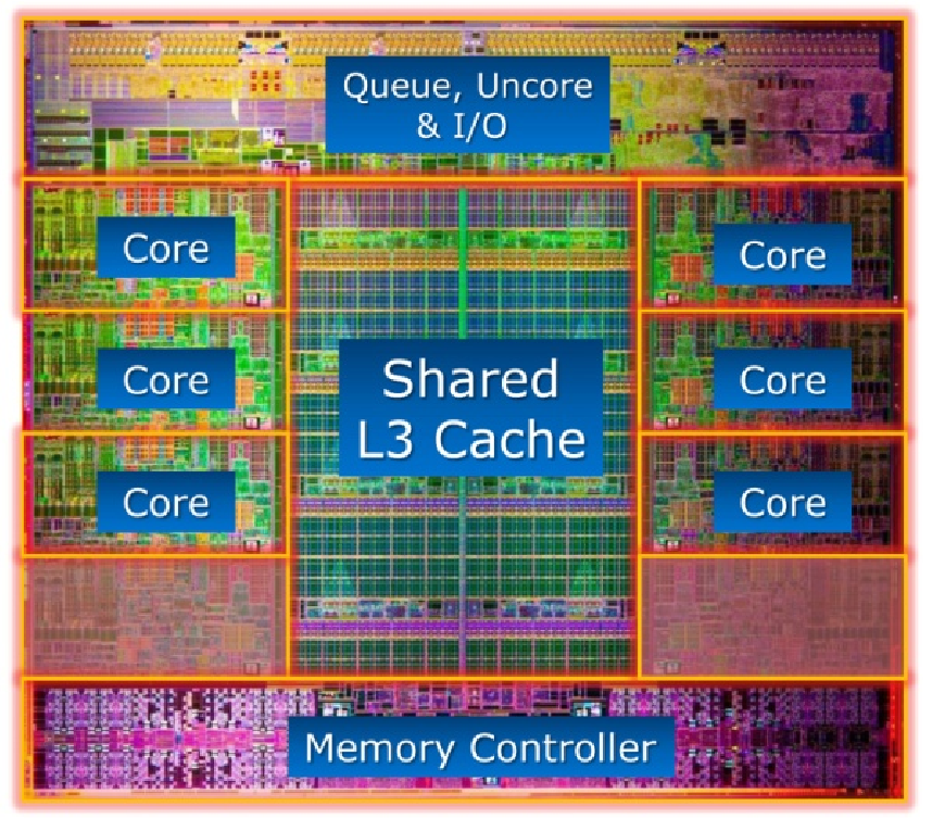
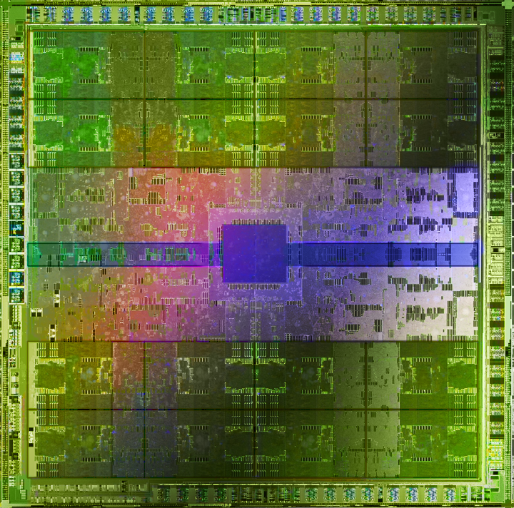
- GPU architecture vs CPU architecture.
- GPUs contain 100s of processing cores on a single card; several cards can fit in a desktop PC
- Each core carries out the same operations in parallel on different input data - single program, multiple data (SPMD) paradigm
- Extremely high arithmetic intensity if one can transfer the data onto and results off of the processors quickly
 |
 |
|---|---|
 |
 |
- From my own experience
- Nvidia cards and its libraries (cuBLAS, cuRAND, cuSparse, ...) are much easier to use than AMD GPUs (OpenCL) for scientific computing.
- Use libraries as much as possible.
- Julia makes life easier: CUBLAS.jl, CUSOLVER.jl, CUSPARSE.jl, ArrayFire.jl, ...
MM example: Netflix and matrix completion
- Snapshot of the kind of data collected by Netflix. Only 100,480,507 ratings (1.2% entries of the 480K-by-18K matrix) are observed
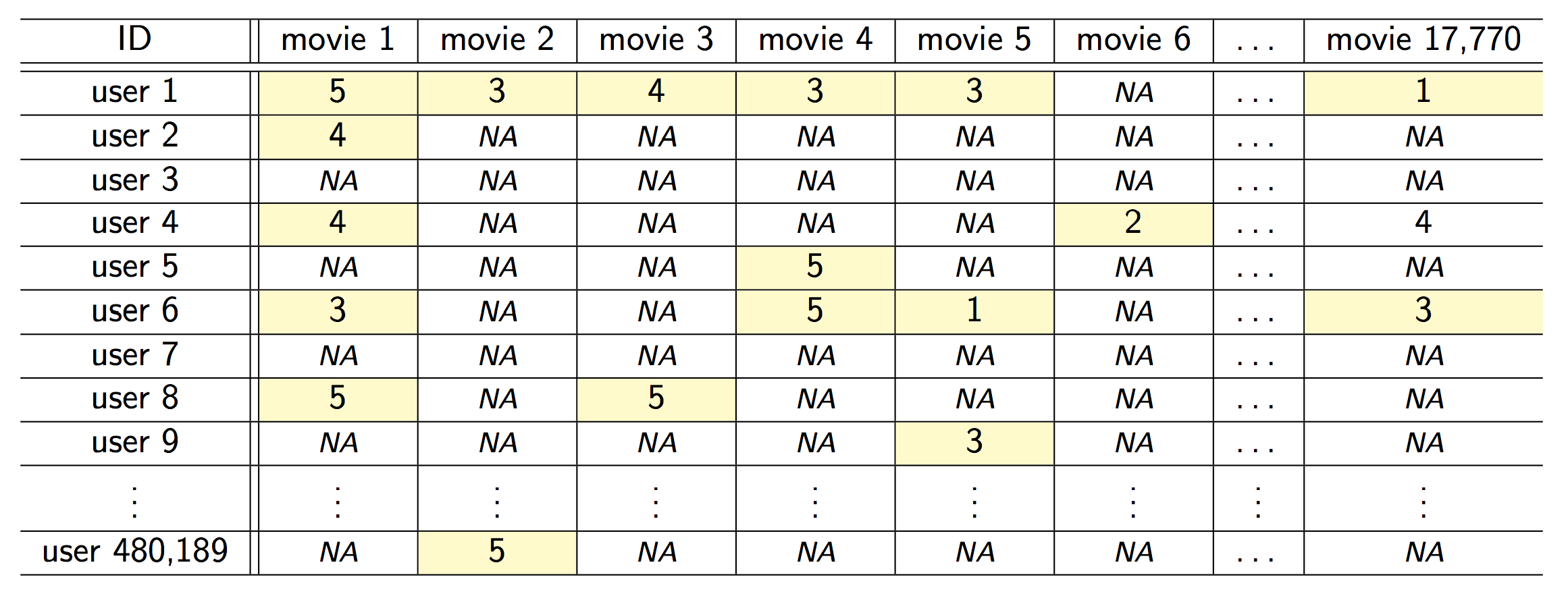
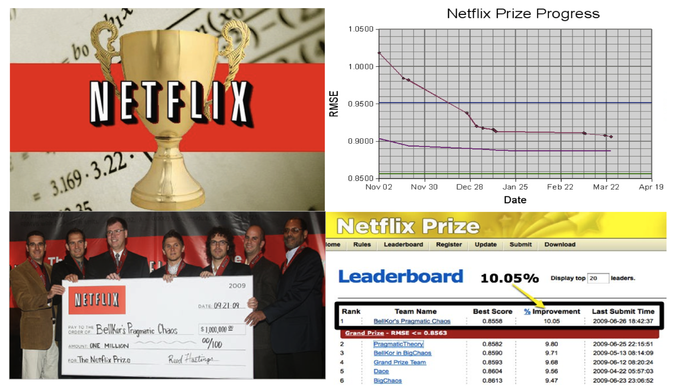
- Netflix challenge: impute the unobserved ratings for personalized recommendation. http://en.wikipedia.org/wiki/Netflix_Prize
Matrix completion problem. Observe a very sparse matrix $\mathbf{Y} = (y_{ij})$. Want to impute all the missing entries. It is possible only when the matrix is structured, e.g., of low rank.
Let $\Omega = \{(i,j): \text{observed entries}\}$ index the set of observed entries and $P_\Omega(\mathbf{M})$ denote the projection of matrix $\mathbf{M}$ to $\Omega$. The problem $$ \min_{\text{rank}(\mathbf{X}) \le r} \frac{1}{2} \| P_\Omega(\mathbf{Y}) - P_\Omega(\mathbf{X})\|_{\text{F}}^2 = \frac{1}{2} \sum_{(i,j) \in \Omega} (y_{ij} - x_{ij})^2 $$ unfortunately is non-convex and difficult.
Convex relaxation: Mazumder, Hastie, Tibshirani (2010) $$ \min_{\mathbf{X}} f(\mathbf{X}) = \frac{1}{2} \| P_\Omega(\mathbf{Y}) - P_\Omega(\mathbf{X})\|_{\text{F}}^2 + \lambda \|\mathbf{X}\|_*, $$ where $\|\mathbf{X}\|_* = \|\sigma(\mathbf{X})\|_1 = \sum_i \sigma_i(\mathbf{X})$ is the nuclear norm.
Majorization step: $$ \begin{eqnarray*} f(\mathbf{X}) &=& \frac{1}{2} \sum_{(i,j) \in \Omega} (y_{ij} - x_{ij})^2 + \frac 12 \sum_{(i,j) \notin \Omega} 0 + \lambda \|\mathbf{X}\|_* \\ &\le& \frac{1}{2} \sum_{(i,j) \in \Omega} (y_{ij} - x_{ij})^2 + \frac{1}{2} \sum_{(i,j) \notin \Omega} (x_{ij}^{(t)} - x_{ij})^2 + \lambda \|\mathbf{X}\|_* \\ &=& \frac{1}{2} \| \mathbf{X} - \mathbf{Z}^{(t)}\|_{\text{F}}^2 + \lambda \|\mathbf{X}\|_* \\ &=& g(\mathbf{X}|\mathbf{X}^{(t)}), \end{eqnarray*} $$ where $\mathbf{Z}^{(t)} = P_\Omega(\mathbf{Y}) + P_{\Omega^\perp}(\mathbf{X}^{(t)})$. "fill in missing entries by the current imputation"
Minimization step:
Rewrite the surrogate function $$ \begin{eqnarray*} g(\mathbf{X}|\mathbf{X}^{(t)}) = \frac{1}{2} \|\mathbf{X}\|_{\text{F}}^2 - \text{tr}(\mathbf{X}^T \mathbf{Z}^{(t)}) + \frac{1}{2} \|\mathbf{Z}^{(t)}\|_{\text{F}}^2 + \lambda \|\mathbf{X}\|_*. \end{eqnarray*} $$ Let $\sigma_i$ be the (ordered) singular values of $\mathbf{X}$ and $\omega_i$ be the (ordered) singular values of $\mathbf{Z}^{(t)}$. Observe $$ \begin{eqnarray*} \|\mathbf{X}\|_{\text{F}}^2 &=& \|\sigma(\mathbf{X})\|_2^2 = \sum_{i} \sigma_i^2 \\ \|\mathbf{Z}^{(t)}\|_{\text{F}}^2 &=& \|\sigma(\mathbf{Z}^{(t)})\|_2^2 = \sum_{i} \omega_i^2 \end{eqnarray*} $$ and by the Fan-von Neuman's inequality $$ \begin{eqnarray*} \text{tr}(\mathbf{X}^T \mathbf{Z}^{(t)}) \le \sum_i \sigma_i \omega_i \end{eqnarray*} $$ with equality achieved if and only if the left and right singular vectors of the two matrices coincide. Thus we should choose $\mathbf{X}$ to have same singular vectors as $\mathbf{Z}^{(t)}$ and $$ \begin{eqnarray*} g(\mathbf{X}|\mathbf{X}^{(t)}) &=& \frac{1}{2} \sum_i \sigma_i^2 - \sum_i \sigma_i \omega_i + \frac{1}{2} \omega_i^2 + \lambda \sum_i \sigma_i \\ &=& \frac{1}{2} \sum_i (\sigma_i - \omega_i)^2 + \lambda \sum_i \sigma_i, \end{eqnarray*} $$ with minimizer given by singular value thresholding $$ \sigma_i^{(t+1)} = (\omega_i - \lambda)_+. $$
Algorithm for matrix completion:
- Initialize $\mathbf{X}^{(0)} \in \mathbb{R}^{m \times n}$
- Repeat
- $\mathbf{Z}^{(t)} \gets P_\Omega(\mathbf{Y}) + P_{\Omega^\perp}(\mathbf{X}^{(t)})$
- Compute SVD: $\mathbf{U} \text{diag}(\mathbf{w}) \mathbf{V}^T \gets \mathbf{Z}^{(t)}$
- $\mathbf{X}^{(t+1)} \gets \mathbf{U} \text{diag}[(\mathbf{w}-\lambda)_+] \mathbf{V}^T$
- objective value converges
"Golub-Kahan-Reinsch" algorithm takes $4m^2n + 8mn^2 + 9n^3$ flops for an $m \ge n$ matrix and is not going to work for 480K-by-18K Netflix matrix.
Notice only top singular values are needed since low rank solutions are achieved by large $\lambda$. Lanczos/Arnoldi algorithm is the way to go. Matrix-vector multiplication $\mathbf{Z}^{(t)} \mathbf{v}$ is fast (why?)