Computer arithmetics
Units of computer storage
bit=binary+digit(coined by statistician John Tukey).byte= 8 bits.- KB = kilobyte = $10^3$ bytes.
- MB = megabytes = $10^6$ bytes.
- GB = gigabytes = $10^9$ bytes. Typical RAM size.
- TB = terabytes = $10^{12}$ bytes. Typical hard drive size. Size of NYSE each trading session.
- PB = petabytes = $10^{15}$ bytes.
- EB = exabytes = $10^{18}$ bytes. Size of all healthcare data in 2011 is ~150 EB.
- ZB = zetabytes = $10^{21}$ bytes.
Julia function Base.summarysize shows the amount of memory (in bytes) used by an object.
x = rand(100, 100)
Base.summarysize(x)
whos() function prints all variables in workspace and their sizes.
whos()
Storage of Characters
- Plain text files are stored in the form of characters:
.jl,.r,.c,.cpp,.ipynb,.html,.tex, ... - ASCII (American Code for Information Interchange): 7 bits, only $2^7=128$ characters.
# integers 0, 1, ..., 127 and corresponding ascii character
# show(STDOUT, "text/plain", [0:127 Char.(0:127)])
[0:127 Char.(0:127)]
- Extended ASCII: 8 bits, $2^8=256$ characters.
# integers 128, 129, ..., 255 and corresponding extended ascii character
# show(STDOUT, "text/plain", [128:255 Char.(128:255)])
[128:255 Char.(128:255)]
Unicode: UTF-8, UTF-16 and UTF-32 support many more characters including foreign characters; last 7 digits conform to ASCII.
UTF-8 is the current dominant character encoding on internet.

- Julia supports the full range of UTF-8 characters. You can type many Unicode math symbols by typing the backslashed LaTeX symbol name followed by tab.
# \beta-<tab>
β = 0.0
# \beta-<tab>-\hat-<tab>
β̂ = 0.0
Fixed-point number system
Fixed-point number system is a computer model for integers $\mathbb{Z}$.
The number of bits and method of representing negative numbers vary from system to system.
- The
integertype in R has $M=32$ or 64 bits. - Matlab has
(u)int8,(u)int16,(u)int32,(u)int64. - Julia has even more integer types. Using Tom Breloff's
Plots.jlandPlotRecipes.jlpackages, we can visualize the type tree underInteger - Storage for a
SignedorUnsignedinteger can be $M = 8, 16, 32, 64$ or 128 bits.
- The
# make a list of a type T and it's supertypes
T = Integer
sups = [T]
sup = T
while sup != Any
    sup = supertype(sup)
    unshift!(sups, sup)
end

# recursively build a graph of subtypes of T
n = length(sups)
nodes, source, destiny = copy(sups), collect(1:n-1), collect(2:n)
function add_subs!(T, supidx)
    for sub in subtypes(T)
        push!(nodes, sub)
        subidx = length(nodes)
        push!(source, supidx)
        push!(destiny, subidx)
        add_subs!(sub, subidx)
    end
end
add_subs!(T, n)
names = map(string, nodes)

using PlotRecipes
#pyplot(alpha=0.5, size=(800, 500))
gr(alpha=0.5, size=(800, 500))
graphplot(source, destiny, names=names, method=:tree)
Signed integers
First bit indicates sign.
0for nonnegative numbers1for negative numbers
Two's complement representation for negative numbers.
- Sign bit is set to 1
- remaining bits are set to opposite values
- 1 is added to the result
- Two's complement representation of a negative integer
xis same as the unsigned integer2^m + x.
@show typeof(18)
@show bits(18)
@show bits(-18)
@show bits(UInt64(Int128(2)^64 - 18)) == bits(-18)
@show bits(2 * 18) # shift bits of 18
@show bits(2 * -18); # shift bits of -18
- Two's complement representation respects modular arithmetic nicely.
Addition of any two signed integers are just bitwise addition, possibly modulo $2^M$

- Range of representable integers by $M$-bit signed integer is $[-2^{M-1},2^{M-1}-1]$.
- Julia functions
typemin(T)andtypemax(T)give the lowest and highest representable number of a typeTrespectively
- Julia functions
for T in [Int8, Int16, Int32, Int64, Int128]
    println(T, '\t', typemin(T), '\t', typemax(T))
end
Unsigned integers
- For unsigned integers, the range is $[0,2^M-1]$.
for t in [UInt8, UInt16, UInt32, UInt64, UInt128]
    println(t, '\t', typemin(t), '\t', typemax(t))
end
BigInt
Julia BigInt type is arbitrary precision.
@show typemax(Int128)
@show typemax(Int128) + 1 # modular arithmetic!
@show BigInt(typemax(Int128)) + 1;
Overflow and underflow for integer arithmetic
R reports NA for integer overflow and underflow.
Julia outputs the result according to modular arithmetic.
@show typemax(Int32)
@show typemax(Int32) + Int32(1); # modular arithmetics!
using RCall

R"""
.Machine$integer.max
"""
R"""
M <- 32
big <- 2^(M-1) - 1
as.integer(big)
"""
R"""
as.integer(big+1)
"""
Floating-number system
Floating-point number system is a computer model for real numbers.
Most computer systems adopt the IEEE 754 standard, established in 1985, for floating-point arithmetics.
For the history, see an interview with William Kahan.In the scientific notation, a real number is represented as $$\pm d_0.d_1d_2 \cdots d_p \times b^e.$$ In computer, the base is $b=2$ and the digits $d_i$ are 0 or 1.
Normalized vs denormalized numbers. For example, decimal number 18 is $$ +1.0010 \times 2^4 \quad (\text{normalized})$$ or, equivalently, $$ +0.1001 \times 2^5 \quad (\text{denormalized}).$$
In the floating-number system, computer stores
- sign bit
- the fraction (or mantissa, or significand) of the normalized representation
- the actual exponent plus a bias
- Double precision (64 bit = 8 bytes)
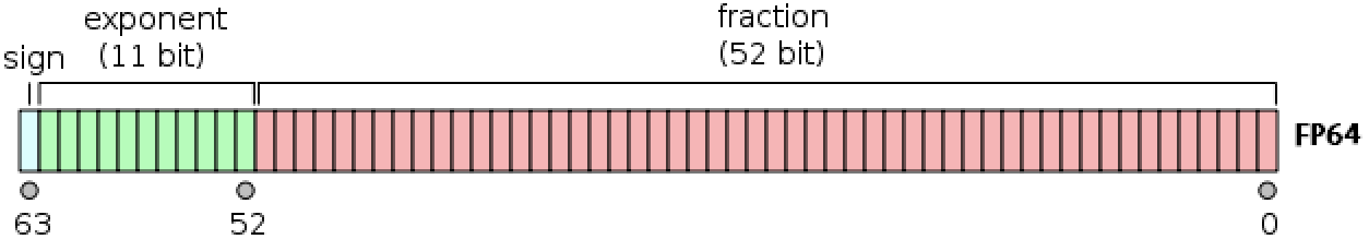
- In Julia,
Float64is the type for double precision numbers - First bit is sign bit
- $p=52$ significant bits
- 11 exponent bits: $e_{\max}=1023$, $e_{\min}=-1022$, bias=1023
- $e_{\text{min}}-1$ and $e_{\text{max}}+1$ are reserved for special numbers
- range of magnitude: $10^{\pm 308}$ in decimal because $\log_{10} (2^{1023}) \approx 308$
- precision to the $\log_{10}(2^{-52}) \approx 16$ decimal point
- In Julia,
Single precision (32 bit = 4 bytes)
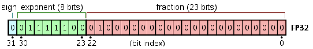
- In Julia,
Float32is the type for single precision numbers - First bit is sign bit
- $p=23$ significant bits
- 8 exponent bits: $e_{\max}=127$, $e_{\min}=-126$, bias=127
- $e_{\text{min}}-1$ and $e_{\text{max}}+1$ are reserved for special numbers
- range of magnitude: $10^{\pm 38}$ in decimal because $\log_{10} (2^{127}) \approx 38$
- precision: $\log_{10}(2^{23}) \approx 7$ decimal point
- In Julia,
Half precision (16 bit = 2 bytes)
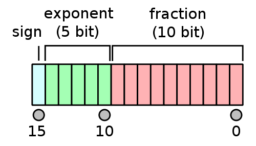
- In Julia,
Float16is the type for half precision numbers - First bit is sign bit
- $p=10$ significant bits
- 5 exponent bits: $e_{\max}=15$, $e_{\min}=-14$, bias=15
- $e_{\text{min}}-1$ and $e_{\text{max}}+1$ are reserved for special numbers
- range of magnitude: $10^{\pm 4}$ in decimal because $\log_{10} (2^{15}) \approx 4$
- precision: $\log_{10}(2^{10}) \approx 3$ decimal point
- In Julia,
println("Half precision:")
@show bits(Float16(18)) # 18 in half precision
@show bits(Float16(-18)) # -18 in half precision
println("Single precision:")
@show bits(Float32(18)) # 18 in single precision
@show bits(Float32(-18)) # -18 in single precision
println("Double precision:")
@show bits(Float64(18)) # 18 in double precision
@show bits(Float64(-18)) # -18 in double precision
@show Float32(π) # SP number displays 7 decimal digits
@show Float64(π) # DP number displays 15 decimal digits
- Special floating-point numbers.
- Exponent $e_{\max}+1$ plus a zero mantissa means $\pm \infty$
- Exponent $e_{\max}+1$ plus a nonzero mantissa means
NaN.NaNcould be produced from0 / 0,0 * Inf, ...
In generalNaN ≠ NaNbitwise - Exponent $e_{\min}-1$ with a zero mantissa represents the real number 0
- Exponent $e_{\min}-1$ with a nonzero mantissa are for numbers less than $b^{e_{\min}}$
Numbers are denormalized in the range $(0,b^{e_{\min}})$ -- graceful underflow
@show bits(Inf) # Inf in double precision
@show bits(-Inf) # -Inf in double precision
@show bits(0 / 0) # NaN
@show bits(0 * Inf) # NaN
@show bits(0.0) # 0 in double precision
@show nextfloat(0.0) # next representable number
@show bits(nextfloat(0.0)); # denormalized
- Rounding is necessary whenever a number has more than $p$ significand bits. Most computer systems use the default IEEE 754 round to nearest mode (also called ties to even mode). Julia offers several rounding modes, the default being
RoundNearest. For example, the number 0.1 in decimal system cannot be represented accurately as a floating point number: $$ 0.1 = 1.10011001... \times 2^{-4} $$
@show bits(0.1f0) # single precision Float32
@show bits(0.1);  # double precision Float64
- In summary
- Single precision: range $\pm 10^{\pm 38}$ with precision up to 7 decimal digits
- Double precision: range $\pm 10^{\pm 308}$ with precision up to 16 decimal digits
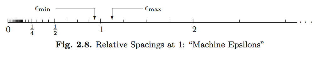
- The floating-point numbers do not occur uniformly over the real number line
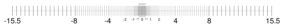 Each magnitude has same number of representible numbers
 - Machine epsilons are the spacings of numbers around 1:
$$\epsilon_{\min}=b^{-p}, \quad \epsilon_{\max} = b^{1-p}.$$
@show eps(Float32)  # machine epsilon for a floating point type
@show eps(Float64)  # same as eps()
# eps(x) is the spacing after x
@show eps(100.0)
@show eps(0.0)
# nextfloat(x) and prevfloat(x) give the neighbors of x
@show x = 1.25f0
@show prevfloat(x), x, nextfloat(x)
@show bits(prevfloat(x)), bits(x), bits(nextfloat(x));
- In R, the variable
.Machinecontains numerical characteristics of the machine.
R"""
.Machine
"""
- Julia provides
Float16(half precision),Float32(single precision),Float64(double precision), andBigFloat(arbitrary precision).
# make a list of a type T and it's supertypes
T = AbstractFloat
sups = [T]
sup = T
while sup != Any
    sup = supertype(sup)
    unshift!(sups,sup)
end
n = length(sups)
nodes, source, destiny = copy(sups), collect(1:n-1), collect(2:n)
add_subs!(T, n)
names = map(string, nodes)

graphplot(source, destiny, names=names, method=:tree)
Overflow and underflow of floating-point number
For double precision, the range is $\pm 10^{\pm 308}$. In most situations, underflow is preferred over overflow. Overflow causes crashes. Underflow yields zeros or denormalized numbers.
E.g., the logit link function is $$p = \frac{\exp (x^T \beta)}{1 + \exp (x^T \beta)} = \frac{1}{1+\exp(- x^T \beta)}.$$ The former expression can easily lead to
Inf / Inf = NaN, while the latter expression leads to graceful underflow.
for T in [Float16, Float32, Float64,]
    println(T, '\t', typemin(T), '\t', typemax(T), '\t', realmin(T),
        '\t', realmax(T), '\t', eps(T))
end
BigFloatin Julia offers arbitrary precision.
@show precision(BigFloat), realmin(BigFloat), realmax(BigFloat);
@show BigFloat(π); # default precision for BigFloat is 256 bits
# set precision to 1024 bits
setprecision(BigFloat, 1024) do
    @show BigFloat(π)
end;
Catastrophic cancellation
- Scenario 1: Addition or subtraction of two numbers of widely different magnitudes: $a+b$ or $a-b$ where $a \gg b$ or $a \ll b$. We loose the precision in the number of smaller magnitude. Consider $$\begin{eqnarray*} a &=& x.xxx ... \times 2^{30} \\ b &=& y.yyy... \times 2^{-30} \end{eqnarray*}$$ What happens when computer calculates $a+b$? We get $a+b=a$!
a = 1.0 * 2.0^30
b = 1.0 * 2.0^-30
a + b == a
- Scenario 2: Subtraction of two nearly equal numbers eliminates significant digits. $a-b$ where $a \approx b$. Consider $$\begin{eqnarray*} a &=& x.xxxxxxxxxx1ssss \\ b &=& x.xxxxxxxxxx0tttt \end{eqnarray*}$$ The result is $1.vvvvu...u$ where $u$ are unassigned digits.
a = 1.2345678f0 # rounding
@show bits(a) # rounding
b = 1.2345677f0
@show bits(b)
@show a - b # correct result should be 1e-7
@show bits(a - b);
- Implications for numerical computation
- Rule 1: add small numbers together before adding larger ones
- Rule 2: add numbers of like magnitude together (paring). When all numbers are of same sign and similar magnitude, add in pairs so each stage the summands are of similar magnitude
- Rule 3: avoid substraction of two numbers that are nearly equal
Algebraic laws
Floating-point numbers may violate many algebraic laws we are familiar with, such associative and distributive laws. See Homework 1 problems.
Further reading
Textbook treatment, e.g., Chapter II.2 of Computational Statistics by James Gentle (2010).
What every computer scientist should know about floating-point arithmetic by David Goldberg (1991).