Cholesky Decomposition

- A basic tenet in numerical analysis:
The structure should be exploited whenever solving a problem.
Common structures include: symmetry, definiteness, sparsity, Kronecker product, low rank, ...
LU decomposition (Gaussian Elimination) is not used in statistics so often because most of time statisticians deal with positive (semi)definite matrix. (That's why I hate to see
solve()in R code.)Consider solving the normal equation $$ \mathbf{X}^T \mathbf{X} \beta = \mathbf{X}^T \mathbf{y} $$ for linear regression. The coefficient matrix $\mathbf{X}^T \mathbf{X}$ is symmetric and positive semidefinite. How to exploit this structure?
Cholesky decomposition
Theorem: Let $\mathbf{A} \in \mathbb{R}^{n \times n}$ be symmetric and positive definite. Then $\mathbf{A} = \mathbf{L} \mathbf{L}^T$, where $\mathbf{L}$ is lower triangular with positive diagonal entries and is unique.
Proof (by induction):
If $n=1$, then $\ell = \sqrt{a}$. For $n>1$, the block equation $$ \begin{eqnarray*} \begin{pmatrix} a_{11} & \mathbf{a}^T \\ \mathbf{a} & \mathbf{A}_{22} \end{pmatrix} = \begin{pmatrix} \ell_{11} & \mathbf{0}_{n-1}^T \\ \mathbf{l} & \mathbf{L}_{22} \end{pmatrix} \begin{pmatrix} \ell_{11} & \mathbf{l}^T \\ \mathbf{0}_{n-1} & \mathbf{L}_{22}^T \end{pmatrix} \end{eqnarray*} $$ has solution $$ \begin{eqnarray*} \ell_{11} &=& \sqrt{a_{11}} \\ \mathbf{l} &=& \ell_{11}^{-1} \mathbf{a} \\ \mathbf{L}_{22} \mathbf{L}_{22}^T &=& \mathbf{A}_{22} - \mathbf{l} \mathbf{l}^T = \mathbf{A}_{22} - a_{11}^{-1} \mathbf{a} \mathbf{a}^T. \end{eqnarray*} $$
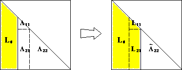
Now $a_{11}>0$ (why?), so $\ell_{11}$ and $\mathbf{l}$ are uniquely determined. $\mathbf{A}_{22} - a_{11}^{-1} \mathbf{a} \mathbf{a}^T$ is positive definite because $\mathbf{A}$ is positive definite (why?). By induction hypothesis, $\mathbf{L}_{22}$ exists and is unique.The constructive proof completely specifies the algorithm:

Computational cost: $$ \frac{1}{2} [2(n-1)^2 + 2(n-2)^2 + \cdots + 2 \cdot 1^2] \approx \frac{1}{3} n^3 \quad \text{flops} $$ plus $n$ square roots. Half the cost of LU decomposition by utilizing symmetry.
In general Cholesky decomposition is very stable. Failure of the decomposition simply means $\mathbf{A}$ is not positive definite. It is an efficient way to test positive definiteness.
Pivoting
When $\mathbf{A}$ does not have full rank, e.g., $\mathbf{X}^T \mathbf{X}$ with a non-full column rank $\mathbf{X}$, we encounter $a_{kk} = 0$ during the procedure.
Symmetric pivoting. At each stage $k$, we permute both row and column such that $\max_{k \le i \le n} a_{ii}$ becomes the pivot. If we encounter $\max_{k \le i \le n} a_{ii} = 0$, then $\mathbf{A}[k:n,k:n] = \mathbf{0}$ (why?) and the algorithm terminates.
With symmetric pivoting: $$ \mathbf{P} \mathbf{A} \mathbf{P}^T = \mathbf{L} \mathbf{L}^T, $$ where $\mathbf{P}$ is a permutation matrix and $\mathbf{L} \in \mathbb{R}^{n \times r}$, $r = \text{rank}(\mathbf{A})$.
Implementation
LAPACK functions:
?potrf(without pivoting),?pstrf(with pivoting).Julia functions:
cholfact,cholfact!,chol, or call LAPACK wrapper functionspotrf!andpstrf!
Example: positive definite matrix.
A = [4 12 -16; 12 37 -43; -16 -43 98]
# Cholesky without pivoting
Achol = cholfact(A)
Achol[:L]
Achol[:U]
b = [1.0; 2.0; 3.0]
A \ b # this does LU; wasteful!; 2/3 n^3 + 2n^2
@which A \ b
Achol \ b # two triangular solves; only 2n^2 flops
@which Achol \ b
det(A) # this actually does LU; wasteful!
@which det(A)
det(Achol) # cheap
@which det(Achol)
inv(A) # this does LU!
@which inv(A)
inv(Achol)
@which inv(Achol)
Example: positive semi-definite matrix.
srand(280) # seed
A = randn(5, 3)
A = A * A'
Achol = cholfact(A)
Achol = cholfact(A, :L, Val{true}) # 3rd argument request partial pivoting
rank(Achol) # determine rank from Cholesky factor
rank(A) # determine rank from SVD, which is more numerically stable
Achol[:L]
Achol[:U]
Achol[:p]
# P A P' = L U
vecnorm(Achol[:P] * A * Achol[:P]' - Achol[:L] * Achol[:U])
Applications
- No inversion mentality: Whenever we see matrix inverse, we should think in terms of solving linear equations. If the matrix is positive (semi)definite, use Cholesky decomposition, which is twice cheaper than LU decomposition.
Multivariate normal density
Multivariate normal density $\text{MVN}(\mu, \Sigma)$, where $\Sigma$ is p.d., is
Method 1: (a) compute explicit inverse $\Sigma^{-1}$ ($2n^3$ flops), (b) compute quadratic form ($2n^2 + 2n$ flops), (c) compute determinant ($2n^3/3$ flops).
Method 2: (a) Cholesky decomposition $\Sigma = \mathbf{L} \mathbf{L}^T$ ($n^3/3$ flops), (b) Solve $\mathbf{L} \mathbf{x} = \mathbf{y} - \mu$ by forward substitutions ($n^2$ flops), (c) compute quadratic form $\mathbf{x}^T \mathbf{x}$ ($2n$ flops), and (d) compute determinant from Cholesky factor ($n$ flops).
Which method is better?
# this is a person w/o any numerical analsyis training
function logpdf_mvn_1(y::Vector, Σ::Matrix)
    n = length(y)
    - (n//2) * log(2π) - (1//2) * logdet(Σ) - (1//2) * y' * inv(Σ) * y
end

# this is an efficiency-savvy person
function logpdf_mvn_2(y::Vector, Σ::Matrix)
    n = length(y)
    Σchol = cholfact(Symmetric(Σ))
    - (n//2) * log(2π) - (1//2) * logdet(Σchol) - (1//2) * sum(abs2, Σchol[:L] \ y)
end

# better memory efficiency
function logpdf_mvn_3(y::Vector, Σ::Matrix)
    n = length(y)
    Σchol = cholfact(Symmetric(Σ))
    - (n//2) * log(2π) - (1//2) * logdet(Σchol) - (1//2) * dot(y, Σchol \ y)
end
using BenchmarkTools, Distributions

srand(280) # seed

n = 1000
Σ = randn(n, n); Σ = Σ' * Σ + I # covariance matrix
y = rand(MvNormal(Σ)) # one randdom sample from N(0, Σ)

# at least they give same answer
@show logpdf_mvn_1(y, Σ)
@show logpdf_mvn_2(y, Σ)
@show logpdf_mvn_3(y, Σ);
@benchmark logpdf_mvn_1(y, Σ)
@benchmark logpdf_mvn_2(y, Σ)
@benchmark logpdf_mvn_3(y, Σ)
- To evaluate same multivariate normal density at many observations $y_1, y_2, \ldots$, we pre-compute the Cholesky decomposition ($n^3/3$ flops), then each evaluation costs $n^2$ flops.
Linear regression
- Cholesky decomposition is one approach to solve linear regression.
- Compute $\mathbf{X}^T \mathbf{X}$: $np^2$ flops
- Compute $\mathbf{X}^T \mathbf{y}$: $2np$ flops
- Cholesky decomposition of $\mathbf{X}^T \mathbf{X}$: $\frac{1}{3} p^3$ flops
- Solve normal equation $\mathbf{X}^T \mathbf{X} \beta = \mathbf{X}^T \mathbf{y}$: $2p^2$ flops
- If need standard errors, another $(4/3)p^3$ flops
Total computational cost is $np^2 + (1/3) p^3$ (without s.e.) or $np^2 + (5/3) p^3$ (with s.e.) flops.
Further reading
Section 7.7 of Numerical Analysis for Statisticians of Kenneth Lange (2010).
Section II.5.3 of Computational Statistics by James Gentle (2010).
Section 4.2 of Matrix Computation by Gene Golub and Charles Van Loan (2013).
versioninfo()