Introduction to Julia

Types of computer languages

  • Compiled languages: C/C++, Fortran, ...

    • Directly compiled to machine code that is executed by CPU
    • Pros: fast, memory efficient
    • Cons: longer development time, hard to debug
  • Interpreted language: R, Matlab, Python, SAS IML, JavaScript, ...

    • Interpreted by interpreter
    • Pros: fast prototyping
    • Cons: excruciatingly slow for loops
  • Mixed (dynamic) languages: Matlab (JIT), R (compiler package), Julia, Cython, JAVA, ...

    • Pros and cons: between the compiled and interpreted languages
  • Script languages: Linux shell scripts, Perl, ...

    • Extremely useful for some data preprocessing and manipulation
  • Database languages: SQL, Hive (Hadoop).

    • Data analysis never happens if we do not know how to retrieve data from databases

Messages

  • To be versatile in the big data era, master at least one language in each category.

  • To improve efficiency of interpreted languages such as R or Matlab, conventional wisdom is to avoid loops as much as possible. Aka, vectorize code

    The only loop you are allowed to have is that for an iterative algorithm.

  • When looping is unavoidable, need to code in C, C++, or Fortran.
    Success stories: the popular glmnet package in R is coded in Fortran; tidyverse packages use a lot RCpp/C++.

  • Modern languages such as Julia tries to solve the two language problem. That is to achieve efficiency without vectorizing code.

What's Julia?

Julia is a high-level, high-performance dynamic programming language for technical computing, with syntax that is familiar to users of other technical computing environments

  • History:

    • Project started in 2009. First public release in 2012
    • Creators: Jeff Bezanson, Alan Edelman, Stefan Karpinski, Viral Shah
    • First major release v1.0 was released on Aug 8, 2018
    • Current stable release v1.1.0
  • Aim to solve the notorious two language problem: Prototype code goes into high-level languages like R/Python, production code goes into low-level language like C/C++.

    Julia aims to:

    Walks like Python. Runs like C.

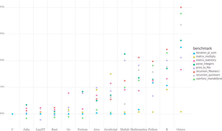
See https://julialang.org/benchmarks/ for the details of benchmark.

  • Write high-level, abstract code that closely resembles mathematical formulas

    • yet produces fast, low-level machine code that has traditionally only been generated by static languages.
  • Julia is more than just "Fast R" or "Fast Matlab"

    • Performance comes from features that work well together.
    • You can't just take the magic dust that makes Julia fast and sprinkle it on [language of choice]
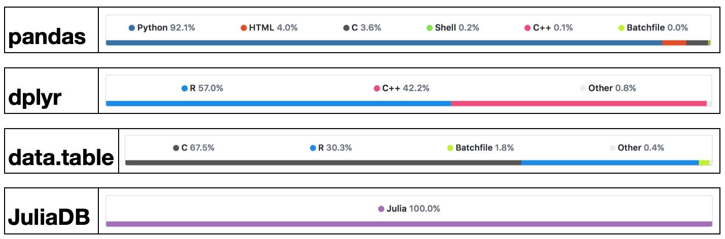
R is great, but...

  • It's not meant for high performance computing

  • Deficiencies in the core language

    • Many fixed with packages (devtools, roxygen2, Matrix)
    • Others harder to fix (R uses an old version of BLAS)
    • Some impossible to fix (clunky syntax, poor design choices)
  • Only 6 active developers left (out of 20 R-Core members)

  • Doug Bates (member of R-Core, Matrix and lme4)

    • Getting Doug on board was a big win for statistics with Julia, as he brought a lot of knowledge about the history of R development and design choices
    • https://github.com/dmbates/MixedModels.jl

      As some of you may know, I have had a (rather late) mid-life crisis and run off with another language called Julia.

      -- Doug Bates (on the `knitr` Google Group)

Gibbs sampler example by Doug Bates

  • An example from Dr. Doug Bates's slides Julia for R Programmers.

  • The task is to create a Gibbs sampler for the density
    $$ f(x, y) = k x^2 exp(- x y^2 - y^2 + 2y - 4x), x > 0 $$ using the conditional distributions $$ \begin{eqnarray*} X | Y &\sim& \Gamma \left( 3, \frac{1}{y^2 + 4} \right) \\ Y | X &\sim& N \left(\frac{1}{1+x}, \frac{1}{2(1+x)} \right). \end{eqnarray*} $$

  • R solution. The RCall.jl package allows us to execute R code without leaving the Julia environment. We first define an R function Rgibbs().
In [1]:
using RCall

R"""
library(Matrix)
Rgibbs <- function(N, thin) {
  mat <- matrix(0, nrow=N, ncol=2)
  x <- y <- 0
  for (i in 1:N) {
    for (j in 1:thin) {
      x <- rgamma(1, 3, y * y + 4) # 3rd arg is rate
      y <- rnorm(1, 1 / (x + 1), 1 / sqrt(2 * (x + 1)))
    }
    mat[i,] <- c(x, y)
  }
  mat
}
"""
Out[1]:
RObject{ClosSxp}
function (N, thin) 
{
    mat <- matrix(0, nrow = N, ncol = 2)
    x <- y <- 0
    for (i in 1:N) {
        for (j in 1:thin) {
            x <- rgamma(1, 3, y * y + 4)
            y <- rnorm(1, 1/(x + 1), 1/sqrt(2 * (x + 1)))
        }
        mat[i, ] <- c(x, y)
    }
    mat
}

To generate a sample of size 10,000 with a thinning of 500. How long does it take?

In [2]:
R"""
system.time(Rgibbs(10000, 500))
"""
Out[2]:
RObject{RealSxp}
   user  system elapsed 
 21.038   2.197  23.265 
  • This is a Julia function for the simple Gibbs sampler:
In [3]:
using Distributions

function jgibbs(N, thin)
    mat = zeros(N, 2)
    x = y = 0.0
    for i in 1:N
        for j in 1:thin
            x = rand(Gamma(3, 1 / (y * y + 4)))
            y = rand(Normal(1 / (x + 1), 1 / sqrt(2(x + 1))))
        end
        mat[i, 1] = x
        mat[i, 2] = y
    end
    mat
end
Out[3]:
jgibbs (generic function with 1 method)

Generate the same number of samples. How long does it take?

In [4]:
jgibbs(100, 5); # warm-up
@elapsed jgibbs(10000, 500)
Out[4]:
0.317547402

We see 40-80 fold speed up of Julia over R on this example, with similar coding effort!

Learning resources

  1. YouTube: Intro to Julia (2h28m), by Jane Herriman.

  2. Cheat sheet: The Fast Track to Julia.

  3. Browse the Julia documentation.

  4. For Matlab users, read Noteworthy Differences From Matlab.

    For R users, read Noteworthy Differences From R.

    For Python users, read Noteworthy Differences From Python.

  5. The Learning page on Julia's website has pointers to many other learning resources.

Julia REPL (Read-Evaluation-Print-Loop)

The Julia REPL, or Julia shell, has at least five modes.

  1. Default mode is the Julian prompt julia>. Type backspace in other modes to enter default mode.

  2. Help mode help?>. Type ? to enter help mode. ?search_term does a fuzzy search for search_term.

  3. Shell mode shell>. Type ; to enter shell mode.

  4. Package mode v(1.1) Pkg>. Type ] to enter package mode for managing Julia packages (install, uninstall, update, ...).

  5. Search mode (reverse-i-search). Press ctrl+R to enter search model.

  6. With RCall.jl package installed, we can enter the R mode by typing $ (shift+4) at Julia REPL.

Some survival commands in Julia REPL:

  1. quit() or Ctrl+D: exit Julia.

  2. Ctrl+C: interrupt execution.

  3. Ctrl+L: clear screen.

  4. Append ; (semi-colon) to suppress displaying output from a command. Same as Matlab.

  5. include("filename.jl") to source a Julia code file.

Seek help

Which IDE?

  • Julia homepage lists many choices: Juno, VS Code, Vim, ...

  • Unfortunately at the moment there are no mature RStudio- or Matlab-like IDE for Julia yet.

  • For dynamic document, e.g., homework, I recommend Jupyter Notebook or JupyterLab. JupyterLab is supposed to replace Jupyter Notebook after it reaches v1.0.

  • For extensive Julia coding, myself has good experience with the editor VS Code with extensions Julia and VS Code Jupyter Notebook Previewer installed.

Julia package system

  • Each Julia package is a Git repository. Each Julia package name ends with .jl. E.g., Distributions.jl package lives at https://github.com/JuliaStats/Distributions.jl.
    Google search with PackageName.jl usually leads to the package on github.com.

  • The package ecosystem is rapidly maturing; a complete list of registered packages (which are required to have a certain level of testing and documentation) is at http://pkg.julialang.org/.

  • For example, the package called Distributions.jl is added with

    # in Pkg mode
    (v1.1) pkg> add Distributions
    

    and "removed" (although not completely deleted) with

    # in Pkg mode
    (v1.1) pkg> rm Distributions
    
  • The package manager provides a dependency solver that determines which packages are actually required to be installed.

  • Non-registered packages are added by cloning the relevant Git repository. E.g.,

    # in Pkg mode
    (v1.1) pkg> add https://github.com/OpenMendel/SnpArrays.jl
    
  • A package needs only be added once, at which point it is downloaded into your local .julia/packages directory in your home directory.

In [5]:
;ls ~/.julia/packages
┌ Warning: special characters "#{}()[]<>|&*?~;" should now be quoted in commands
│   caller = #shell_parse#351(::String, ::Function, ::String, ::Bool) at shell.jl:100
└ @ Base ./shell.jl:100
AbstractFFTs
AccurateArithmetic
AlgorithmsFromTheBook
Arpack
AssetRegistry
AxisAlgorithms
AxisArrays
BEDFiles
BenchmarkTools
BinDeps
BinaryProvider
Blink
BufferedStreams
CMake
CMakeWrapper
CSSUtil
CSTParser
CSV
Cairo
Calculus
CatIndices
CategoricalArrays
Cbc
Clp
Clustering
CodecBzip2
CodecXz
CodecZlib
CodecZstd
Codecs
ColorTypes
ColorVectorSpace
Colors
CommonSubexpressions
Compat
Compose
ComputationalResources
Conda
Contour
Convex
CoordinateTransformations
CoupledFields
CustomUnitRanges
DataArrays
DataFrames
DataStreams
DataStructures
DataValues
DecFP
DecisionTree
DeepDiffs
DiffEqDiffTools
DiffResults
DiffRules
Distances
Distributions
DocStringExtensions
Documenter
DocumenterTools
DoubleFloats
ECOS
EzXML
FFTViews
FFTW
FactCheck
FileIO
FilePaths
FilePathsBase
FixedPointNumbers
Fontconfig
ForwardDiff
FunctionalCollections
GLM
GLPK
GLPKMathProgInterface
GR
GZip
Gadfly
GenericLinearAlgebra
Glob
Graphics
Gurobi
HTTP
HTTPClient
Hexagons
Hiccup
Highlights
Homebrew
HttpCommon
HttpParser
IJulia
IdentityRanges
ImageAxes
ImageCore
ImageDistances
ImageFiltering
ImageMagick
ImageMetadata
ImageMorphology
ImageShow
ImageTransformations
Images
IndirectArrays
IniFile
Interact
InteractBase
InteractBulma
InternedStrings
Interpolations
IntervalSets
Ipopt
IterTools
IterableTables
IterativeSolvers
IteratorInterfaceExtensions
JLD2
JSExpr
JSON
JuMP
Juno
KernelDensity
Knockout
LaTeXStrings
Lazy
LibCURL
LibExpat
Libz
LinQuadOptInterface
LineSearches
LinearMaps
Literate
Loess
MATLAB
MPI
MacroTools
MappedArrays
MathOptInterface
MathProgBase
MbedTLS
Measures
Media
MendelPlots
Missings
Mocking
Mosek
Mustache
Mux
NLSolversBase
NLopt
NaNMath
NamedTuples
NearestNeighbors
NodeJS
Nullables
ORCA
Observables
OffsetArrays
Optim
OptimTestProblems
OrderedCollections
OrdinalGWAS
OrdinalMultinomialModels
PDMats
PaddedViews
Parameters
Parsers
Pidfile
PlotReferenceImages
PlotThemes
PlotUtils
Plotly
PlotlyBase
PlotlyJS
Plots
PolrGWAS
PolrModels
Polynomials
PooledArrays
PositiveFactorizations
Primes
ProgressMeter
PyCall
PyPlot
QuadGK
QuartzImageIO
RCall
RData
RDatasets
RangeArrays
Ratios
RecipesBase
RecursiveArrayTools
Reexport
Requests
Requires
ReverseDiffSparse
Rmath
Roots
Rotations
Rsvg
SCS
SIUnits
ScikitLearnBase
ShowItLikeYouBuildIt
Showoff
SimpleTraits
SnpArrays
SoftGlobalScope
SortingAlgorithms
SpecialFunctions
StatPlots
StaticArrays
StatsBase
StatsFuns
StatsModels
StatsPlots
Suppressor
TableShowUtils
TableTraits
TableTraitsUtils
Tables
TestImages
TestSetExtensions
TexExtensions
TextParse
TiledIteration
TimeZones
Tokenize
TranscodingStreams
URIParser
UnicodePlots
VarianceComponentModels
VarianceComponentTest
VegaDatasets
VegaLite
VersionParsing
VisualRegressionTests
WeakRefStrings
Weave
WebIO
WebSockets
Widgets
WinRPM
WinReg
WoodburyMatrices
YAML
ZMQ
ZipFile
  • Directory of a specific package can be queried by pathof():
In [6]:
using Distributions

pathof(Distributions)
Out[6]:
"/Users/huazhou/.julia/packages/Distributions/fMt8c/src/Distributions.jl"
  • If you start having problems with packages that seem to be unsolvable, you may try just deleting your .julia directory and reinstalling all your packages.

  • Periodically, one should run update in Pkg mode, which checks for, downloads and installs updated versions of all the packages you currently have installed.

  • status lists the status of all installed packages.

  • Using functions in package.

    using Distributions
    

    This pulls all of the exported functions in the module into your local namespace, as you can check using the whos() command. An alternative is

    import Distributions
    

    Now, the functions from the Distributions package are available only using

    Distributions.<FUNNAME>
    

    All functions, not only exported functions, are always available like this.

Calling R from Julia

  • The RCall.jl package allows us to embed R code inside of Julia.

  • There are also PyCall.jl, MATLAB.jl, JavaCall.jl, CxxWrap.jl packages for interfacing with other languages.

In [7]:
using RCall

x = randn(1000)
R"""
hist($x, main="I'm plotting a Julia vector")
"""
Out[7]:
RObject{VecSxp}
$breaks
 [1] -5 -4 -3 -2 -1  0  1  2  3  4

$counts
[1]   1   0  28 119 369 320 142  19   2

$density
[1] 0.001 0.000 0.028 0.119 0.369 0.320 0.142 0.019 0.002

$mids
[1] -4.5 -3.5 -2.5 -1.5 -0.5  0.5  1.5  2.5  3.5

$xname
[1] "`#JL`$x"

$equidist
[1] TRUE

attr(,"class")
[1] "histogram"
In [8]:
R"""
library(ggplot2)
qplot($x)
"""
Out[8]:
RObject{VecSxp}
┌ Warning: RCall.jl: `stat_bin()` using `bins = 30`. Pick better value with `binwidth`.
└ @ RCall /Users/huazhou/.julia/packages/RCall/ffM0W/src/io.jl:113
In [9]:
x = R"""
rnorm(10)
"""
Out[9]:
RObject{RealSxp}
 [1] -1.76152465  0.28402321 -1.18674201  0.38532610  0.66327415 -0.07548059
 [7] -1.22814518 -0.36132394 -1.58982131  1.00019919
In [10]:
# collect R variable into Julia workspace
y = collect(x)
Out[10]:
10-element Array{Float64,1}:
 -1.761524654252555  
  0.2840232126371199 
 -1.1867420051409112 
  0.38532610091816666
  0.6632741501853096 
 -0.07548059232008238
 -1.2281451847872713 
 -0.36132394376250476
 -1.589821307258373  
  1.0001991932779424 
  • Access Julia variables in R REPL mode:

    julia> x = rand(5) # Julia variable
    R> y <- $x
    
  • Pass Julia expression in R REPL mode:

    R> y <- $(rand(5))
    
  • Put Julia variable into R environment:

    julia> @rput x
    R> x
    
  • Get R variable into Julia environment:

    R> r <- 2
    Julia> @rget r
    
  • If you want to call Julia within R, check out the XRJulia package by John Chambers.

Some basic Julia code

In [11]:
# an integer, same as int in R
y = 1
typeof(y)
Out[11]:
Int64
In [12]:
# a Float64 number, same as double in R
y = 1.0
typeof(y)
Out[12]:
Float64
In [13]:
# Greek letters:  `\pi<tab>`
π
Out[13]:
π = 3.1415926535897...
In [14]:
typeof(π)
Out[14]:
Irrational{:π}
In [15]:
# Greek letters:  `\theta<tab>`
θ = y + π
Out[15]:
4.141592653589793
In [16]:
# emoji! `\:kissing_cat:<tab>`
😽 = 5.0
Out[16]:
5.0
In [17]:
# `\alpha<tab>\hat<tab>`
α̂ = π
Out[17]:
π = 3.1415926535897...
In [18]:
# vector of Float64 0s
x = zeros(5)
Out[18]:
5-element Array{Float64,1}:
 0.0
 0.0
 0.0
 0.0
 0.0
In [19]:
# vector Int64 0s
x = zeros(Int, 5)
Out[19]:
5-element Array{Int64,1}:
 0
 0
 0
 0
 0
In [20]:
# matrix of Float64 0s
x = zeros(5, 3)
Out[20]:
5×3 Array{Float64,2}:
 0.0  0.0  0.0
 0.0  0.0  0.0
 0.0  0.0  0.0
 0.0  0.0  0.0
 0.0  0.0  0.0
In [21]:
# matrix of Float64 1s
x = ones(5, 3)
Out[21]:
5×3 Array{Float64,2}:
 1.0  1.0  1.0
 1.0  1.0  1.0
 1.0  1.0  1.0
 1.0  1.0  1.0
 1.0  1.0  1.0
In [22]:
# define array without initialization
x = Matrix{Float64}(undef, 5, 3)
Out[22]:
5×3 Array{Float64,2}:
 2.353e-314    2.35072e-314  2.33123e-314
 2.353e-314    2.33123e-314  0.0         
 2.33123e-314  2.34943e-314  0.0         
 2.34943e-314  2.33123e-314  0.0         
 2.35132e-314  2.33123e-314  0.0         
In [23]:
# fill a matrix by 0s
fill!(x, 0)
Out[23]:
5×3 Array{Float64,2}:
 0.0  0.0  0.0
 0.0  0.0  0.0
 0.0  0.0  0.0
 0.0  0.0  0.0
 0.0  0.0  0.0
In [24]:
# initialize an array to be constant 2.5
fill(2.5, (5, 3))
Out[24]:
5×3 Array{Float64,2}:
 2.5  2.5  2.5
 2.5  2.5  2.5
 2.5  2.5  2.5
 2.5  2.5  2.5
 2.5  2.5  2.5
In [25]:
# rational number
a = 3//5
Out[25]:
3//5
In [26]:
typeof(a)
Out[26]:
Rational{Int64}
In [27]:
b = 3//7
Out[27]:
3//7
In [28]:
a + b
Out[28]:
36//35
In [29]:
# uniform [0, 1) random numbers
x = rand(5, 3)
Out[29]:
5×3 Array{Float64,2}:
 0.697832  0.521255  0.635389
 0.795756  0.821073  0.046378
 0.330146  0.200252  0.997733
 0.12915   0.951122  0.227358
 0.833891  0.494311  0.428478
In [30]:
# uniform random numbers (in single precision)
x = rand(Float16, 5, 3)
Out[30]:
5×3 Array{Float16,2}:
 0.8604  0.798   0.1611
 0.717   0.4043  0.0762
 0.5312  0.0742  0.8906
 0.2373  0.1309  0.632 
 0.5137  0.42    0.5244
In [31]:
# random numbers from {1,...,5}
x = rand(1:5, 5, 3)
Out[31]:
5×3 Array{Int64,2}:
 1  4  5
 2  2  2
 5  2  3
 2  3  5
 1  1  1
In [32]:
# standard normal random numbers
x = randn(5, 3)
Out[32]:
5×3 Array{Float64,2}:
  1.14235   -0.681071    0.360989
  1.95432   -0.0724878   0.329729
 -0.288511  -1.22229     1.32657 
 -0.774164   1.37268    -1.37873 
 -0.2116     0.861211   -1.25181 
In [33]:
# range
1:10
Out[33]:
1:10
In [34]:
typeof(1:10)
Out[34]:
UnitRange{Int64}
In [35]:
1:2:10
Out[35]:
1:2:9
In [36]:
typeof(1:2:10)
Out[36]:
StepRange{Int64,Int64}
In [37]:
# integers 1-10
x = collect(1:10)
Out[37]:
10-element Array{Int64,1}:
  1
  2
  3
  4
  5
  6
  7
  8
  9
 10
In [38]:
# or equivalently
[1:10...]
Out[38]:
10-element Array{Int64,1}:
  1
  2
  3
  4
  5
  6
  7
  8
  9
 10
In [39]:
# Float64 numbers 1-10
x = collect(1.0:10)
Out[39]:
10-element Array{Float64,1}:
  1.0
  2.0
  3.0
  4.0
  5.0
  6.0
  7.0
  8.0
  9.0
 10.0
In [40]:
# convert to a specific type
convert(Vector{Float64}, 1:10)
Out[40]:
10-element Array{Float64,1}:
  1.0
  2.0
  3.0
  4.0
  5.0
  6.0
  7.0
  8.0
  9.0
 10.0

Timing and benchmark

Julia

@time, @elapsed, @allocated macros:

In [41]:
using Random # standard library
Random.seed!(123) # seed
x = rand(1_000_000) # 1 million random numbers in [0, 1)

@time sum(x) # first run includes compilation time
  0.032345 seconds (95.66 k allocations: 4.858 MiB)
Out[41]:
500060.34072352527
In [42]:
@time sum(x) # no compilation time after first run
  0.000456 seconds (5 allocations: 176 bytes)
Out[42]:
500060.34072352527
In [43]:
# just the runtime
@elapsed sum(x)
Out[43]:
0.000449506
In [44]:
# just the allocation
@allocated sum(x)
Out[44]:
16

Use package BenchmarkTools.jl for more robust benchmarking. Analog of microbenchmark package in R.

In [45]:
using BenchmarkTools

bm = @benchmark sum($x)
Out[45]:
BenchmarkTools.Trial: 
  memory estimate:  0 bytes
  allocs estimate:  0
  --------------
  minimum time:     244.108 μs (0.00% GC)
  median time:      268.166 μs (0.00% GC)
  mean time:        280.042 μs (0.00% GC)
  maximum time:     2.854 ms (0.00% GC)
  --------------
  samples:          10000
  evals/sample:     1
In [46]:
using Statistics # standard library
benchmark_result = Dict() # a dictionary to store median runtime (in milliseconds)
benchmark_result["Julia builtin"] = median(bm.times) / 1e6
Out[46]:
0.2681655

C

We would use the low-level C code as the baseline for copmarison. In Julia, we can easily run compiled C code using the ccall function.

In [47]:
using Libdl

C_code = """
#include <stddef.h>
double c_sum(size_t n, double *X) {
    double s = 0.0;
    for (size_t i = 0; i < n; ++i) {
        s += X[i];
    }
    return s;
}
"""

const Clib = tempname()   # make a temporary file

# compile to a shared library by piping C_code to gcc
# (works only if you have gcc installed):

open(`gcc -std=c99 -fPIC -O3 -msse3 -xc -shared -o $(Clib * "." * Libdl.dlext) -`, "w") do f
    print(f, C_code) 
end

# define a Julia function that calls the C function:
c_sum(X::Array{Float64}) = ccall(("c_sum", Clib), Float64, (Csize_t, Ptr{Float64}), length(X), X)
Out[47]:
c_sum (generic function with 1 method)
In [48]:
# make sure it gives same answer
c_sum(x)
Out[48]:
500060.340723512
In [49]:
bm = @benchmark c_sum($x)
Out[49]:
BenchmarkTools.Trial: 
  memory estimate:  0 bytes
  allocs estimate:  0
  --------------
  minimum time:     1.117 ms (0.00% GC)
  median time:      1.134 ms (0.00% GC)
  mean time:        1.161 ms (0.00% GC)
  maximum time:     3.056 ms (0.00% GC)
  --------------
  samples:          4297
  evals/sample:     1
In [50]:
# store median runtime (in milliseconds)
benchmark_result["C"] = median(bm.times) / 1e6
Out[50]:
1.134183

R, buildin sum

Next we compare to the build in sum function in R, which is implemented using C.

In [51]:
using RCall

R"""
library(microbenchmark)
y <- $x
rbm <- microbenchmark(sum(y))
"""
Out[51]:
RObject{VecSxp}
Unit: microseconds
   expr     min      lq     mean  median       uq      max neval
 sum(y) 897.061 902.984 978.2313 995.058 1006.212 1239.114   100
In [52]:
# store median runtime (in milliseconds)
@rget rbm # dataframe
benchmark_result["R builtin"] = median(rbm[:time]) / 1e6
Out[52]:
0.995058

R, handwritten loop

Handwritten loop in R is much slower.

In [53]:
using RCall

R"""
sum_r <- function(x) {
  s <- 0
  for (xi in x) {
    s <- s + xi
  }
  s
}
library(microbenchmark)
y <- $x
rbm <- microbenchmark(sum_r(y))
"""
Out[53]:
RObject{VecSxp}
Unit: milliseconds
     expr      min       lq     mean   median       uq      max neval
 sum_r(y) 25.42925 26.79393 27.30556 27.21291 27.72341 33.88999   100
In [54]:
# store median runtime (in milliseconds)
@rget rbm # dataframe
benchmark_result["R loop"] = median(rbm[:time]) / 1e6
Out[54]:
27.212913

Python, builtin sum

Built in function sum in Python.

In [55]:
using PyCall
PyCall.pyversion
Out[55]:
v"3.7.3"
In [56]:
# get the Python built-in "sum" function:
pysum = pybuiltin("sum")
bm = @benchmark $pysum($x)
Out[56]:
BenchmarkTools.Trial: 
  memory estimate:  368 bytes
  allocs estimate:  8
  --------------
  minimum time:     81.864 ms (0.00% GC)
  median time:      83.359 ms (0.00% GC)
  mean time:        83.663 ms (0.00% GC)
  maximum time:     89.594 ms (0.00% GC)
  --------------
  samples:          60
  evals/sample:     1
In [57]:
# store median runtime (in miliseconds)
benchmark_result["Python builtin"] = median(bm.times) / 1e6
Out[57]:
83.3590615

Python, handwritten loop

In [58]:
using PyCall

py"""
def py_sum(A):
    s = 0.0
    for a in A:
        s += a
    return s
"""

sum_py = py"py_sum"

bm = @benchmark $sum_py($x)
Out[58]:
BenchmarkTools.Trial: 
  memory estimate:  368 bytes
  allocs estimate:  8
  --------------
  minimum time:     96.864 ms (0.00% GC)
  median time:      101.652 ms (0.00% GC)
  mean time:        101.390 ms (0.00% GC)
  maximum time:     109.707 ms (0.00% GC)
  --------------
  samples:          50
  evals/sample:     1
In [59]:
# store median runtime (in miliseconds)
benchmark_result["Python loop"] = median(bm.times) / 1e6
Out[59]:
101.652003

Python, numpy

Numpy is the high-performance scientific computing library for Python.

In [60]:
# bring in sum function from Numpy 
numpy_sum = pyimport("numpy")."sum"
Out[60]:
PyObject <function sum at 0x128308b70>
In [61]:
bm = @benchmark $numpy_sum($x)
Out[61]:
BenchmarkTools.Trial: 
  memory estimate:  368 bytes
  allocs estimate:  8
  --------------
  minimum time:     303.052 μs (0.00% GC)
  median time:      336.714 μs (0.00% GC)
  mean time:        357.059 μs (0.00% GC)
  maximum time:     2.370 ms (0.00% GC)
  --------------
  samples:          10000
  evals/sample:     1
In [62]:
# store median runtime (in miliseconds)
benchmark_result["Python numpy"] = median(bm.times) / 1e6
Out[62]:
0.336714

Numpy performance is on a par with Julia build-in sum function. Both are about 3 times faster than C, possibly because of usage of SIMD.

Summary

In [63]:
benchmark_result
Out[63]:
Dict{Any,Any} with 7 entries:
  "R builtin"      => 0.995058
  "Julia builtin"  => 0.268166
  "Python builtin" => 83.3591
  "C"              => 1.13418
  "Python loop"    => 101.652
  "Python numpy"   => 0.336714
  "R loop"         => 27.2129
  • C and R builtin are the baseline C performance (gold standard).

  • Python builtin and Python loop are 80-100 fold slower than C because the loop is interpreted.

  • R loop is about 30 folder slower than C and indicates the performance of bytecode generated by its compiler package (turned on by default since R v3.4.0 (Apr 2017)).

  • Julia builtin and Python numpy are 3-4 folder faster than C because of SIMD (???).

Matrices and vectors

Dimensions

In [64]:
x = randn(5, 3)
Out[64]:
5×3 Array{Float64,2}:
  0.598655   -0.649164  -0.20795  
 -1.50715     1.41208    0.29778  
 -2.08909     0.283026  -1.37727  
  0.0489631   2.06727   -0.0209721
 -0.0975634  -0.194017   0.133924 
In [65]:
size(x)
Out[65]:
(5, 3)
In [66]:
size(x, 1) # nrow() in R
Out[66]:
5
In [67]:
size(x, 2)
Out[67]:
3
In [68]:
# total number of elements
length(x)
Out[68]:
15

Indexing

In [69]:
# 5 × 5 matrix of random Normal(0, 1)
x = randn(5, 5)
Out[69]:
5×5 Array{Float64,2}:
  1.40584   -0.435559  -1.77228    0.616302   0.979726  
 -0.434523   0.986161   0.942634  -1.27926   -1.15752   
  0.643141   0.39562    0.396688  -0.220179  -0.841993  
 -1.23652   -1.03567   -1.227     -1.13857   -1.86035   
  0.528711  -1.36271   -0.387252   0.79865    0.00320293
In [70]:
# first column
x[:, 1]
Out[70]:
5-element Array{Float64,1}:
  1.405836567860699 
 -0.4345229408667341
  0.6431414215485608
 -1.2365159892763888
  0.5287106504891519
In [71]:
# first row
x[1, :]
Out[71]:
5-element Array{Float64,1}:
  1.405836567860699 
 -0.4355593559026318
 -1.7722776947141923
  0.6163015601209474
  0.9797260369028392
In [72]:
# sub-array
x[1:2, 2:3]
Out[72]:
2×2 Array{Float64,2}:
 -0.435559  -1.77228 
  0.986161   0.942634
In [73]:
# getting a subset of a matrix creates a copy, but you can also create "views"
z = view(x, 1:2, 2:3)
Out[73]:
2×2 view(::Array{Float64,2}, 1:2, 2:3) with eltype Float64:
 -0.435559  -1.77228 
  0.986161   0.942634
In [74]:
# same as
@views z = x[1:2, 2:3]
Out[74]:
2×2 view(::Array{Float64,2}, 1:2, 2:3) with eltype Float64:
 -0.435559  -1.77228 
  0.986161   0.942634
In [75]:
# change in z (view) changes x as well
z[2, 2] = 0.0
x
Out[75]:
5×5 Array{Float64,2}:
  1.40584   -0.435559  -1.77228    0.616302   0.979726  
 -0.434523   0.986161   0.0       -1.27926   -1.15752   
  0.643141   0.39562    0.396688  -0.220179  -0.841993  
 -1.23652   -1.03567   -1.227     -1.13857   -1.86035   
  0.528711  -1.36271   -0.387252   0.79865    0.00320293
In [76]:
# y points to same data as x
y = x
Out[76]:
5×5 Array{Float64,2}:
  1.40584   -0.435559  -1.77228    0.616302   0.979726  
 -0.434523   0.986161   0.0       -1.27926   -1.15752   
  0.643141   0.39562    0.396688  -0.220179  -0.841993  
 -1.23652   -1.03567   -1.227     -1.13857   -1.86035   
  0.528711  -1.36271   -0.387252   0.79865    0.00320293
In [77]:
# x and y point to same data
pointer(x), pointer(y)
Out[77]:
(Ptr{Float64} @0x000000011a458050, Ptr{Float64} @0x000000011a458050)
In [78]:
# changing y also changes x
y[:, 1] .= 0
x
Out[78]:
5×5 Array{Float64,2}:
 0.0  -0.435559  -1.77228    0.616302   0.979726  
 0.0   0.986161   0.0       -1.27926   -1.15752   
 0.0   0.39562    0.396688  -0.220179  -0.841993  
 0.0  -1.03567   -1.227     -1.13857   -1.86035   
 0.0  -1.36271   -0.387252   0.79865    0.00320293
In [79]:
# create a new copy of data
z = copy(x)
Out[79]:
5×5 Array{Float64,2}:
 0.0  -0.435559  -1.77228    0.616302   0.979726  
 0.0   0.986161   0.0       -1.27926   -1.15752   
 0.0   0.39562    0.396688  -0.220179  -0.841993  
 0.0  -1.03567   -1.227     -1.13857   -1.86035   
 0.0  -1.36271   -0.387252   0.79865    0.00320293
In [80]:
pointer(x), pointer(z)
Out[80]:
(Ptr{Float64} @0x000000011a458050, Ptr{Float64} @0x000000011a458950)

Concatenate matrices

In [81]:
# 1-by-3 array
[1 2 3]
Out[81]:
1×3 Array{Int64,2}:
 1  2  3
In [82]:
# 3-by-1 vector
[1, 2, 3]
Out[82]:
3-element Array{Int64,1}:
 1
 2
 3
In [83]:
# multiple assignment by tuple
x, y, z = randn(5, 3), randn(5, 2), randn(3, 5)
Out[83]:
([1.07455 2.55508 1.26546; 0.385123 -0.660738 -1.64513; … ; -0.583523 0.43622 0.385691; 0.832241 -1.32354 0.177505], [-0.997382 -0.488503; -0.817314 0.673586; … ; -1.39357 0.729497; 0.53823 0.57519], [-2.30427 1.62085 … 0.054552 0.49251; 1.3284 -1.14737 … 0.167511 -1.1699; -0.908365 0.423386 … -1.26891 0.883105])
In [84]:
[x y] # 5-by-5 matrix
Out[84]:
5×5 Array{Float64,2}:
  1.07455    2.55508    1.26546   -0.997382  -0.488503
  0.385123  -0.660738  -1.64513   -0.817314   0.673586
 -2.38285   -0.693591  -0.465704   0.605258   0.302012
 -0.583523   0.43622    0.385691  -1.39357    0.729497
  0.832241  -1.32354    0.177505   0.53823    0.57519 
In [85]:
[x y; z] # 8-by-5 matrix
Out[85]:
8×5 Array{Float64,2}:
  1.07455    2.55508    1.26546    -0.997382  -0.488503
  0.385123  -0.660738  -1.64513    -0.817314   0.673586
 -2.38285   -0.693591  -0.465704    0.605258   0.302012
 -0.583523   0.43622    0.385691   -1.39357    0.729497
  0.832241  -1.32354    0.177505    0.53823    0.57519 
 -2.30427    1.62085   -0.0751243   0.054552   0.49251 
  1.3284    -1.14737   -0.121207    0.167511  -1.1699  
 -0.908365   0.423386  -0.163381   -1.26891    0.883105

Dot operation

Dot operation in Julia is elementwise operation, similar to Matlab.

In [86]:
x = randn(5, 3)
Out[86]:
5×3 Array{Float64,2}:
  1.42693     1.1571     0.352857
  0.270257   -0.17928    0.137277
 -0.0178663  -1.02672   -0.321545
  0.865855   -0.232668   1.1365  
  0.0332832   0.886387  -1.66359 
In [87]:
y = ones(5, 3)
Out[87]:
5×3 Array{Float64,2}:
 1.0  1.0  1.0
 1.0  1.0  1.0
 1.0  1.0  1.0
 1.0  1.0  1.0
 1.0  1.0  1.0
In [88]:
x .* y # same x * y in R
Out[88]:
5×3 Array{Float64,2}:
  1.42693     1.1571     0.352857
  0.270257   -0.17928    0.137277
 -0.0178663  -1.02672   -0.321545
  0.865855   -0.232668   1.1365  
  0.0332832   0.886387  -1.66359 
In [89]:
x .^ (-2)
Out[89]:
5×3 Array{Float64,2}:
    0.491126   0.746898   8.0316  
   13.6914    31.1127    53.0649  
 3132.79       0.948625   9.67199 
    1.33386   18.4725     0.774221
  902.711      1.27278    0.361334
In [90]:
sin.(x)
Out[90]:
5×3 Array{Float64,2}:
  0.98967     0.91564    0.34558 
  0.266979   -0.178321   0.136846
 -0.0178653  -0.855607  -0.316033
  0.76165    -0.230575   0.907164
  0.0332771   0.774793  -0.995698

Basic linear algebra

In [91]:
x = randn(5)
Out[91]:
5-element Array{Float64,1}:
 -0.48876941581527183
 -1.8898912365052984 
  0.4752801478661729 
  0.5986586722127957 
  1.8129740483514514 
In [92]:
using LinearAlgebra
# vector L2 norm
norm(x)
Out[92]:
2.77159570508093
In [93]:
# same as
sqrt(sum(abs2, x))
Out[93]:
2.77159570508093
In [94]:
y = randn(5) # another vector
# dot product
dot(x, y) # x' * y
Out[94]:
-2.0757729618710195
In [95]:
# same as
x'y
Out[95]:
-2.0757729618710195
In [96]:
x, y = randn(5, 3), randn(3, 2)
# matrix multiplication, same as %*% in R
x * y
Out[96]:
5×2 Array{Float64,2}:
 -0.159807   0.579995
  0.621269   1.32793 
  0.591513  -1.99637 
 -0.713616   0.684772
 -0.557596   0.75847 
In [97]:
x = randn(3, 3)
Out[97]:
3×3 Array{Float64,2}:
  0.153422   1.0588      0.277495
  0.271558   0.0482019   0.326489
 -1.21251   -0.0983329  -0.623121
In [98]:
# conjugate transpose
x'
Out[98]:
3×3 Adjoint{Float64,Array{Float64,2}}:
 0.153422  0.271558   -1.21251  
 1.0588    0.0482019  -0.0983329
 0.277495  0.326489   -0.623121 
In [99]:
b = rand(3)
x'b # same as x' * b
Out[99]:
3-element Array{Float64,1}:
 -0.8462924095954427 
  0.46434157973051327
 -0.1889119302892237 
In [100]:
# trace
tr(x)
Out[100]:
-0.4214969667533476
In [101]:
det(x)
Out[101]:
-0.2308584804640239
In [102]:
rank(x)
Out[102]:
3

Sparse matrices

In [103]:
using SparseArrays

# 10-by-10 sparse matrix with sparsity 0.1
X = sprandn(10, 10, .1)
Out[103]:
10×10 SparseMatrixCSC{Float64,Int64} with 10 stored entries:
  [6 ,  1]  =  -0.251681
  [5 ,  2]  =  -0.778148
  [9 ,  4]  =  -0.119565
  [2 ,  5]  =  -0.616153
  [7 ,  5]  =  -1.40975
  [2 ,  7]  =  0.84617
  [7 ,  7]  =  -0.207459
  [9 ,  8]  =  -0.0429563
  [5 ,  9]  =  -0.388533
  [2 , 10]  =  -0.209722
In [104]:
# convert to dense matrix; be cautious when dealing with big data
Xfull = convert(Matrix{Float64}, X)
Out[104]:
10×10 Array{Float64,2}:
  0.0        0.0       0.0   0.0       …   0.0         0.0        0.0     
  0.0        0.0       0.0   0.0           0.0         0.0       -0.209722
  0.0        0.0       0.0   0.0           0.0         0.0        0.0     
  0.0        0.0       0.0   0.0           0.0         0.0        0.0     
  0.0       -0.778148  0.0   0.0           0.0        -0.388533   0.0     
 -0.251681   0.0       0.0   0.0       …   0.0         0.0        0.0     
  0.0        0.0       0.0   0.0           0.0         0.0        0.0     
  0.0        0.0       0.0   0.0           0.0         0.0        0.0     
  0.0        0.0       0.0  -0.119565     -0.0429563   0.0        0.0     
  0.0        0.0       0.0   0.0           0.0         0.0        0.0     
In [105]:
# convert a dense matrix to sparse matrix
sparse(Xfull)
Out[105]:
10×10 SparseMatrixCSC{Float64,Int64} with 10 stored entries:
  [6 ,  1]  =  -0.251681
  [5 ,  2]  =  -0.778148
  [9 ,  4]  =  -0.119565
  [2 ,  5]  =  -0.616153
  [7 ,  5]  =  -1.40975
  [2 ,  7]  =  0.84617
  [7 ,  7]  =  -0.207459
  [9 ,  8]  =  -0.0429563
  [5 ,  9]  =  -0.388533
  [2 , 10]  =  -0.209722
In [106]:
# syntax for sparse linear algebra is same as dense linear algebra
β = ones(10)
X * β
Out[106]:
10-element Array{Float64,1}:
  0.0                
  0.02029443774752057
  0.0                
  0.0                
 -1.1666816429212037 
 -0.25168069117368247
 -1.617210771834139  
  0.0                
 -0.1625211385544279 
  0.0                
In [107]:
# many functions apply to sparse matrices as well
sum(X)
Out[107]:
-3.177799806735933

Control flow and loops

  • if-elseif-else-end
if condition1
    # do something
elseif condition2
    # do something
else
    # do something
end
  • for loop
for i in 1:10
    println(i)
end
  • Nested for loop:
for i in 1:10
    for j in 1:5
        println(i * j)
    end
end

Same as

for i in 1:10, j in 1:5
    println(i * j)
end
  • Exit loop:
for i in 1:10
    # do something
    if condition1
        break # skip remaining loop
    end
end
  • Exit iteration:
for i in 1:10
    # do something
    if condition1
        continue # skip to next iteration
    end
    # do something
end

Functions

  • In Julia, all arguments to functions are passed by reference, in contrast to R and Matlab.

  • Function names ending with ! indicates that function mutates at least one argument, typically the first.

    sort!(x) # vs sort(x)
    
  • Function definition

function func(req1, req2; key1=dflt1, key2=dflt2)
    # do stuff
    return out1, out2, out3
end

Required arguments are separated with a comma and use the positional notation.
Optional arguments need a default value in the signature.
Semicolon is not required in function call.
return statement is optional.
Multiple outputs can be returned as a tuple, e.g., return out1, out2, out3.

  • Anonymous functions, e.g., x -> x^2, is commonly used in collection function or list comprehensions.

    map(x -> x^2, y) # square each element in x
    
  • Functions can be nested:

function outerfunction()
    # do some outer stuff
    function innerfunction()
        # do inner stuff
        # can access prior outer definitions
    end
    # do more outer stuff
end
  • Functions can be vectorized using the Dot syntax:
In [108]:
function myfunc(x)
    return sin(x^2)
end

x = randn(5, 3)
myfunc.(x)
Out[108]:
5×3 Array{Float64,2}:
  0.639626   0.0671957   0.275807  
  0.139496   0.387134    0.414554  
  0.721616   0.00984144  0.79227   
 -0.633982  -0.556283    0.0602744 
  0.544461   0.156409    0.00768604
  • Collection function (think this as the series of apply functions in R).

    Apply a function to each element of a collection:

map(f, coll) # or
map(coll) do elem
    # do stuff with elem
    # must contain return
end
In [109]:
map(x -> sin(x^2), x)
Out[109]:
5×3 Array{Float64,2}:
  0.639626   0.0671957   0.275807  
  0.139496   0.387134    0.414554  
  0.721616   0.00984144  0.79227   
 -0.633982  -0.556283    0.0602744 
  0.544461   0.156409    0.00768604
In [110]:
map(x) do elem
    elem = elem^2
    return sin(elem)
end
Out[110]:
5×3 Array{Float64,2}:
  0.639626   0.0671957   0.275807  
  0.139496   0.387134    0.414554  
  0.721616   0.00984144  0.79227   
 -0.633982  -0.556283    0.0602744 
  0.544461   0.156409    0.00768604
In [111]:
# Mapreduce
mapreduce(x -> sin(x^2), +, x)
Out[111]:
3.026104609456178
In [112]:
# same as
sum(x -> sin(x^2), x)
Out[112]:
3.026104609456178
  • List comprehension
In [113]:
[sin(2i + j) for i in 1:5, j in 1:3] # similar to Python
Out[113]:
5×3 Array{Float64,2}:
  0.14112   -0.756802  -0.958924
 -0.958924  -0.279415   0.656987
  0.656987   0.989358   0.412118
  0.412118  -0.544021  -0.99999 
 -0.99999   -0.536573   0.420167

Type system

  • Every variable in Julia has a type.

  • When thinking about types, think about sets.

  • Everything is a subtype of the abstract type Any.

  • An abstract type defines a set of types

    • Consider types in Julia that are a Number:

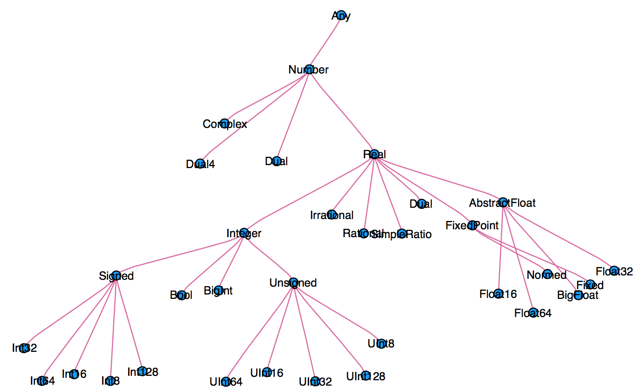
  • We can explore type hierarchy with typeof(), supertype(), and subtypes().
In [114]:
typeof(1.0), typeof(1)
Out[114]:
(Float64, Int64)
In [115]:
supertype(Float64)
Out[115]:
AbstractFloat
In [116]:
subtypes(AbstractFloat)
Out[116]:
4-element Array{Any,1}:
 BigFloat
 Float16 
 Float32 
 Float64 
In [117]:
# Is Float64 a subtype of AbstractFloat?
Float64 <: AbstractFloat
Out[117]:
true
In [118]:
# On 64bit machine, Int == Int64
Int == Int64
Out[118]:
true
In [119]:
# convert to Float64
convert(Float64, 1)
Out[119]:
1.0
In [120]:
# same as
Float64(1)
Out[120]:
1.0
In [121]:
# Float32 vector
x = randn(Float32, 5)
Out[121]:
5-element Array{Float32,1}:
 -0.27314892
 -1.4175588 
  0.06751722
 -2.4249308 
 -0.9561249 
In [122]:
# convert to Float64
convert(Vector{Float64}, x)
Out[122]:
5-element Array{Float64,1}:
 -0.27314892411231995
 -1.4175587892532349 
  0.0675172209739685 
 -2.4249308109283447 
 -0.9561249017715454 
In [123]:
# same as
Float64.(x)
Out[123]:
5-element Array{Float64,1}:
 -0.27314892411231995
 -1.4175587892532349 
  0.0675172209739685 
 -2.4249308109283447 
 -0.9561249017715454 
In [124]:
# convert Float64 to Int64
convert(Int, 1.0)
Out[124]:
1
In [125]:
convert(Int, 1.5) # should use round(1.5)
InexactError: Int64(1.5)

Stacktrace:
 [1] Type at ./float.jl:703 [inlined]
 [2] convert(::Type{Int64}, ::Float64) at ./number.jl:7
 [3] top-level scope at In[125]:1
In [126]:
round(Int, 1.5)
Out[126]:
2

Multiple dispatch

  • Multiple dispatch lies in the core of Julia design. It allows built-in and user-defined functions to be overloaded for different combinations of argument types.

  • Let's consider a simple "doubling" function:

In [127]:
g(x) = x + x
Out[127]:
g (generic function with 1 method)
In [128]:
g(1.5)
Out[128]:
3.0

This definition is too broad, since some things, e.g., strings, can't be added

In [129]:
g("hello world")
MethodError: no method matching +(::String, ::String)
Closest candidates are:
  +(::Any, ::Any, !Matched::Any, !Matched::Any...) at operators.jl:502
  +(!Matched::PyObject, ::Any) at /Users/huazhou/.julia/packages/PyCall/a5Jd3/src/pyoperators.jl:13
  +(::Any, !Matched::PyObject) at /Users/huazhou/.julia/packages/PyCall/a5Jd3/src/pyoperators.jl:14

Stacktrace:
 [1] g(::String) at ./In[127]:1
 [2] top-level scope at In[129]:1
  • This definition is correct but too restrictive, since any Number can be added.
In [130]:
g(x::Float64) = x + x
Out[130]:
g (generic function with 2 methods)
  • This definition will automatically work on the entire type tree above!
In [131]:
g(x::Number) = x + x
Out[131]:
g (generic function with 3 methods)

This is a lot nicer than

function g(x)
    if isa(x, Number)
        return x + x
    else
        throw(ArgumentError("x should be a number"))
    end
end
  • methods(func) function display all methods defined for func.
In [132]:
methods(g)
Out[132]:
3 methods for generic function g:
  • g(x::Float64) in Main at In[130]:1
  • g(x::Number) in Main at In[131]:1
  • g(x) in Main at In[127]:1
  • When calling a function with multiple definitions, Julia will search from the narrowest signature to the broadest signature.

  • @which func(x) marco tells which method is being used for argument signature x.

In [133]:
# an Int64 input
@which g(1)
Out[133]:
g(x::Number) in Main at In[131]:1
In [134]:
# a Vector{Float64} input
@which g(randn(5))
Out[134]:
g(x) in Main at In[127]:1

Just-in-time compilation (JIT)

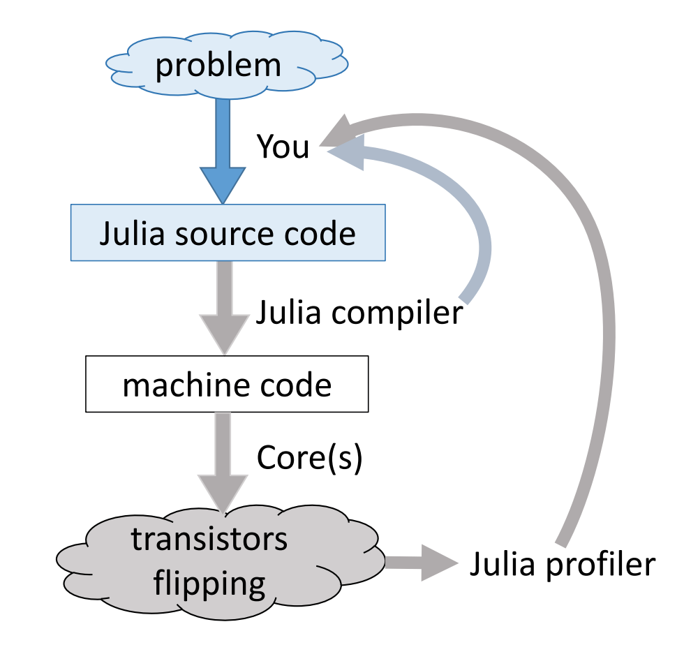
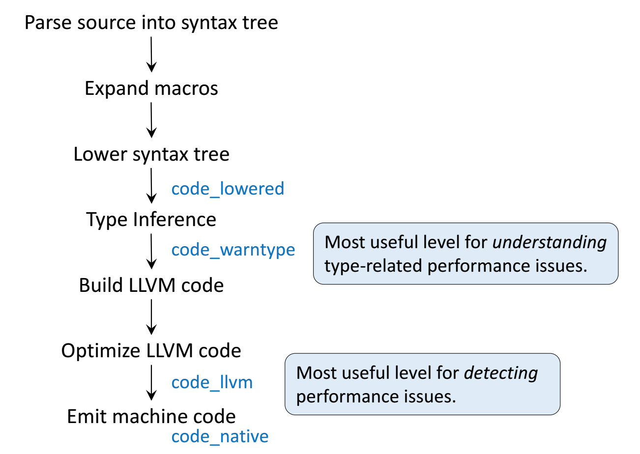
Following figures are taken from Arch D. Robinson's slides Introduction to Writing High Performance Julia.

Julia toolchain Julia toolchain
  • Julia's efficiency results from its capability to infer the types of all variables within a function and then call LLVM to generate optimized machine code at run-time.

Consider the g (doubling) function defined earlier. This function will work on any type which has a method for +.

In [135]:
g(2), g(2.0)
Out[135]:
(4, 4.0)

Step 1: Parse Julia code into abstract syntax tree (AST).

In [136]:
@code_lowered g(2)
Out[136]:
CodeInfo(
1 ─ %1 = x + x
└──      return %1
)

Step 2: Type inference according to input type.

In [137]:
@code_warntype g(2)
Body::Int64
1 ─ %1 = (Base.add_int)(x, x)::Int64
└──      return %1
In [138]:
@code_warntype g(2.0)
Body::Float64
1 ─ %1 = (Base.add_float)(x, x)::Float64
└──      return %1

Step 3: Compile into LLVM bytecode (equivalent of R bytecode generated by compiler package).

In [139]:
@code_llvm g(2)
;  @ In[131]:1 within `g'
define i64 @julia_g_15080(i64) {
top:
; ┌ @ int.jl:53 within `+'
   %1 = shl i64 %0, 1
; └
  ret i64 %1
}
In [140]:
@code_llvm g(2.0)
;  @ In[130]:1 within `g'
define double @julia_g_15081(double) {
top:
; ┌ @ float.jl:395 within `+'
   %1 = fadd double %0, %0
; └
  ret double %1
}

We didn't provide a type annotation. But different LLVM code gets generated depending on the argument type!

In R or Python, g(2) and g(2.0) would use the same code for both.

In Julia, g(2) and g(2.0) dispatches to optimized code for Int64 and Float64, respectively.

For integer input x, LLVM compiler is smart enough to know x + x is simple shifting x by 1 bit, which is faster than addition.

  • Step 4: Lowest level is the assembly code, which is machine dependent.
In [141]:
@code_native g(2)
	.section	__TEXT,__text,regular,pure_instructions
; ┌ @ In[131]:1 within `g'
; │┌ @ In[131]:1 within `+'
	decl	%eax
	leal	(%edi,%edi), %eax
; │└
	retl
	nopw	%cs:(%eax,%eax)
; └
In [142]:
@code_native g(2.0)
	.section	__TEXT,__text,regular,pure_instructions
; ┌ @ In[130]:1 within `g'
; │┌ @ In[130]:1 within `+'
	vaddsd	%xmm0, %xmm0, %xmm0
; │└
	retl
	nopw	%cs:(%eax,%eax)
; └

Profiling Julia code

Julia has several built-in tools for profiling. The @time marco outputs run time and heap allocation.

In [143]:
# a function defined earlier
function tally(x::Array)
    s = zero(eltype(x))
    for v in x
        s += v
    end
    s
end

using Random
Random.seed!(123)
a = rand(20_000_000)
@time tally(a) # first run: include compile time
  0.036713 seconds (5.84 k allocations: 276.576 KiB)
Out[143]:
1.0000233387279043e7
In [144]:
@time tally(a)
  0.026384 seconds (5 allocations: 176 bytes)
Out[144]:
1.0000233387279043e7

For more robust benchmarking, the BenchmarkTools.jl package is highly recommended.

In [145]:
using BenchmarkTools

@benchmark tally($a)
Out[145]:
BenchmarkTools.Trial: 
  memory estimate:  0 bytes
  allocs estimate:  0
  --------------
  minimum time:     21.450 ms (0.00% GC)
  median time:      23.802 ms (0.00% GC)
  mean time:        23.774 ms (0.00% GC)
  maximum time:     29.245 ms (0.00% GC)
  --------------
  samples:          211
  evals/sample:     1

The Profile module gives line by line profile results.

In [146]:
using Profile

Profile.clear()
@profile tally(a)
Profile.print(format=:flat)
 Count File                        Line Function                               
    23 ./In[143]                      5 tally(::Array{Float64,1})              
    25 ./boot.jl                    328 eval                                   
     1 ./broadcast.jl               551 _broadcast_getindex(::Base.Broadcast...
     1 ./broadcast.jl               578 _broadcast_getindex                    
     1 ./broadcast.jl               578 _broadcast_getindex_evalf(::typeof(S...
     1 ./broadcast.jl               791 copy                                   
     1 ./broadcast.jl               791 copy(::Base.Broadcast.Broadcasted{Ba...
     2 ./broadcast.jl               928 copyto_nonleaf!(::Array{Expr,1}, ::B...
     2 ./broadcast.jl               511 getindex                               
     2 ./broadcast.jl               753 materialize(::Base.Broadcast.Broadca...
    26 ./essentials.jl              742 #invokelatest#1                        
    26 ./essentials.jl              741 invokelatest                           
    23 ./float.jl                   395 +                                      
    26 ./task.jl                    259 (::getfield(IJulia, Symbol("##15#18"...
    26 .../9ajf8/src/eventloop.jl     8 eventloop(::ZMQ.Socket)                
    26 .../src/execute_request.jl    67 execute_request(::ZMQ.Socket, ::IJul...
     2 .../src/SoftGlobalScope.jl   124 _softscope                             
     1 .../src/SoftGlobalScope.jl   144 _softscope(::Expr, ::Set{Symbol}, ::...
     1 .../src/SoftGlobalScope.jl   152 _softscope(::Expr, ::Set{Symbol}, ::...
     1 .../src/SoftGlobalScope.jl   154 _softscope(::Expr, ::Set{Symbol}, ::...
     1 .../src/SoftGlobalScope.jl   177 softscope(::Module, ::Expr)            
     1 .../src/SoftGlobalScope.jl   217 softscope_include_string(::Module, :...
    25 .../src/SoftGlobalScope.jl   218 softscope_include_string(::Module, :...

One can use ProfileView package for better visualization of profile data:

using ProfileView

ProfileView.view()

Memory profiling

Detailed memory profiling requires a detour. First let's write a script bar.jl, which contains the workload function tally and a wrapper for profiling.

In [147]:
;cat bar.jl
using Profile

function tally(x::Array)
    s = zero(eltype(x))
    for v in x
        s += v
    end
    s
end

# call workload from wrapper to avoid misattribution bug
function wrapper()
    y = rand(10000)
    # force compilation
    println(tally(y))
    # clear allocation counters
    Profile.clear_malloc_data()
    # run compiled workload
    println(tally(y))
end

wrapper()

Next, in terminal, we run the script with --track-allocation=user option.

In [148]:
;julia --track-allocation=user bar.jl
5012.163648117665
5012.163648117665

The profiler outputs a file bar.jl.21740.mem.

In [149]:
;cat bar.jl.21740.mem
        - using Profile
        - 
        - function tally(x::Array)
        -     s = zero(eltype(x))
        -     for v in x
        -         s += v
        -     end
        -     s
        - end
        - 
        - # call workload from wrapper to avoid misattribution bug
        - function wrapper()
        0     y = rand(10000)
        -     # force compilation
        0     println(tally(y))
        -     # clear allocation counters
        0     Profile.clear_malloc_data()
        -     # run compiled workload
      144     println(tally(y))
        - end
        - 
        - wrapper()
        -