Convexity, Duality, and Optimality Conditions (KL Chapter 11, BV Chapter 5)
Convexity
A function $f: \mathbb{R}^n \mapsto \mathbb{R}$ is convex if
- $\text{dom} f$ is a convex set: $\lambda \mathbf{x} + (1-\lambda) \mathbf{y} \in \text{dom} f$ for all $\mathbf{x},\mathbf{y} \in \text{dom} f$ and any $\lambda \in (0, 1)$, and
- $f(\lambda \mathbf{x} + (1-\lambda) \mathbf{y}) \le \lambda f(\mathbf{x}) + (1-\lambda) f(\mathbf{y})$, for all $\mathbf{x},\mathbf{y} \in \text{dom} f$ and $\lambda \in (0,1)$.
$f$ is strictly convex if the inequality is strict for all $\mathbf{x} \ne \mathbf{y} \in \text{dom} f$ and $\lambda$.
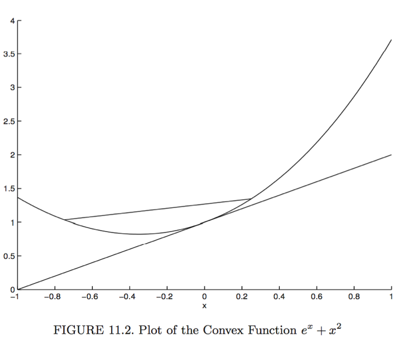
Supporting hyperplane inequality. A differentiable function $f$ is convex if and only if $$ f(\mathbf{x}) \ge f(\mathbf{y}) + \nabla f(\mathbf{y})^T (\mathbf{x}-\mathbf{y}) $$ for all $\mathbf{x}, \mathbf{y} \in \text{dom} f$.
Second-order condition for convexity. A twice differentiable function $f$ is convex if and only if $\nabla^2f(\mathbf{x})$ is psd for all $\mathbf{x} \in \text{dom} f$. It is strictly convex if and only if $\nabla^2f(\mathbf{x})$ is pd for all $\mathbf{x} \in \text{dom} f$.
Convexity and global optima. Suppose $f$ is a convex function.
- Any stationary point $\mathbf{y}$, i.e., $\nabla f(\mathbf{y})=\mathbf{0}$, is a global minimum. (Proof: By supporting hyperplane inequality, $f(\mathbf{x}) \ge f(\mathbf{y}) + \nabla f(\mathbf{y})^T (\mathbf{x} - \mathbf{y}) = f(\mathbf{y})$ for all $\mathbf{x} \in \text{dom} f$.)
- Any local minimum is a global minimum.
- The set of (global) minima is convex.
- If $f$ is strictly convex, then the global minimum, if exists, is unique.
Example: Least squares estimate. $f(\beta) = \frac 12 \| \mathbf{y} - \mathbf{X} \beta \|_2^2$ has Hessian $\nabla^2f = \mathbf{X}^T \mathbf{X}$ which is psd. So $f$ is convex and any stationary point (solution to the normal equation) is a global minimum. When $\mathbf{X}$ is rank deficient, the set of solutions is convex.
Jensen's inequality. If $h$ is convex and $\mathbf{W}$ a random vector taking values in $\text{dom} f$, then $$ \mathbf{E}[h(\mathbf{W})] \ge h [\mathbf{E}(\mathbf{W})], $$ provided both expectations exist. For a strictly convex $h$, equality holds if and only if $W = \mathbf{E}(W)$ almost surely.
Proof: Take $\mathbf{x} = \mathbf{W}$ and $\mathbf{y} = \mathbf{E} (\mathbf{W})$ in the supporting hyperplane inequality.
Information inequality. Let $f$ and $g$ be two densities with respect to a common measure $\mu$ and $f, g>0$ almost everywhere relative to $\mu$. Then $$ \mathbf{E}_f (\log f) \ge \mathbf{E}_f (\log g), $$ with equality if and only if $f = g$ almost everywhere on $\mu$.
Proof: Apply Jensen's inequality to the convex function $- \ln(t)$ and random variable $W=g(X)/f(X)$ where $X \sim f$.
Important applications of information inequality: M-estimation, EM algorithm.
Duality
Consider optimization problem \begin{eqnarray*} &\text{minimize}& f_0(\mathbf{x}) \\ &\text{subject to}& f_i(\mathbf{x}) \le 0, \quad i = 1,\ldots,m \\ & & h_i(\mathbf{x}) = 0, \quad i = 1,\ldots,p. \end{eqnarray*}
The Lagrangian is \begin{eqnarray*} L(\mathbf{x}, \lambda, \nu) = f_0(\mathbf{x}) + \sum_{i=1}^m \lambda_i f_i(\mathbf{x}) + \sum_{i=1}^p \nu_i h_i(\mathbf{x}). \end{eqnarray*} The vectors $\lambda = (\lambda_1,\ldots, \lambda_m)^T$ and $\nu = (\nu_1,\ldots,\nu_p)^T$ are called the Lagrange multiplier vectors or dual variables.
The Lagrange dual function is the minimum value of the Langrangian over $\mathbf{x}$ \begin{eqnarray*} g(\lambda, \mu) = \inf_{\mathbf{x}} L(\mathbf{x}, \lambda, \nu) = \inf_{\mathbf{x}} \left( f_0(\mathbf{x}) + \sum_{i=1}^m \lambda_i f_i(\mathbf{x}) + \sum_{i=1}^p \nu_i h_i(\mathbf{x}) \right). \end{eqnarray*}
Denote the optimal value of original problem by $p^\star$. For any $\lambda \succeq \mathbf{0}$ and any $\nu$, we have \begin{eqnarray*} g(\lambda, \nu) \le p^\star. \end{eqnarray*} Proof: For any feasible point $\tilde{\mathbf{x}}$, \begin{eqnarray*} L(\tilde{\mathbf{x}}, \lambda, \nu) = f_0(\tilde{\mathbf{x}}) + \sum_{i=1}^m \lambda_i f_i(\tilde{\mathbf{x}}) + \sum_{i=1}^p \nu_i h_i(\tilde{\mathbf{x}}) \le f_0(\tilde{\mathbf{x}}) \end{eqnarray*} because the second term is non-positive and the third term is zero. Then \begin{eqnarray*} g(\lambda, \mu) = \inf_{\mathbf{x}} L(\mathbf{x}, \lambda, \mu) \le L(\tilde{\mathbf{x}}, \lambda, \nu) \le f_0(\tilde{\mathbf{x}}). \end{eqnarray*}
Since each pair $(\lambda, \nu)$ with $\lambda \succeq \mathbf{0}$ gives a lower bound to the optimal value $p^\star$. It is natural to ask for the best possible lower bound the Lagrange dual function can provide. This leads to the Lagrange dual problem \begin{eqnarray*} &\text{maximize}& g(\lambda, \nu) \\ &\text{subject to}& \lambda \succeq \mathbf{0}, \end{eqnarray*} which is a convex problem regardless the primal problem is convex or not.
We denote the optimal value of the Lagrange dual problem by $d^\star$, which satifies the week duality \begin{eqnarray*} d^\star \le p^\star. \end{eqnarray*} The difference $p^\star - d^\star$ is called the optimal duality gap.
If the primal problem is convex, that is \begin{eqnarray*} &\text{minimize}& f_0(\mathbf{x}) \\ &\text{subject to}& f_i(\mathbf{x}) \le 0, \quad i = 1,\ldots,m \\ & & \mathbf{A} \mathbf{x} = \mathbf{b}, \end{eqnarray*} with $f_0,\ldots,f_m$ convex, we usually (but not always) have the strong duality, i.e., $d^\star = p^\star$.
The conditions under which strong duality holds are called constraint qualifications. A commonly used one is Slater's condition: There exists a point in the relative interior of the domain such that \begin{eqnarray*} f_i(\mathbf{x}) < 0, \quad i = 1,\ldots,m, \quad \mathbf{A} \mathbf{x} = \mathbf{b}. \end{eqnarray*} Such a point is also called strictly feasible.
KKT optimality conditions
KKT is "one of the great triumphs of 20th century applied mathematics" (KL Chapter 11).
Nonconvex problems
Assume $f_0,\ldots,f_m,h_1,\ldots,h_p$ are differentiable. Let $\mathbf{x}^\star$ and $(\lambda^\star, \nu^\star)$ be any primal and dual optimal points with zero duality gap, i.e., strong duality holds.
Since $\mathbf{x}^\star$ minimizes $L(\mathbf{x}, \lambda^\star, \nu^\star)$ over $\mathbf{x}$, its gradient vanishes at $\mathbf{x}^\star$, we have the Karush-Kuhn-Tucker (KKT) conditions \begin{eqnarray*} f_i(\mathbf{x}^\star) &\le& 0, \quad i = 1,\ldots,m \\ h_i(\mathbf{x}^\star) &=& 0, \quad i = 1,\ldots,p \\ \lambda_i^\star &\ge& 0, \quad i = 1,\ldots,m \\ \lambda_i^\star f_i(\mathbf{x}^\star) &=& 0, \quad i=1,\ldots,m \\ \nabla f_0(\mathbf{x}^\star) + \sum_{i=1}^m \lambda_i^\star \nabla f_i(\mathbf{x}^\star) + \sum_{i=1}^p \nu_i^\star \nabla h_i(\mathbf{x}^\star) &=& \mathbf{0}. \end{eqnarray*}
The fourth condition (complementary slackness) follows from \begin{eqnarray*} f_0(\mathbf{x}^\star) &=& g(\lambda^\star, \nu^\star) \\ &=& \inf_{\mathbf{x}} \left( f_0(\mathbf{x}) + \sum_{i=1}^m \lambda_i^\star f_i(\mathbf{x}) + \sum_{i=1}^p \nu_i^\star h_i(\mathbf{x}) \right) \\ &\le& f_0(\mathbf{x}^\star) + \sum_{i=1}^m \lambda_i^\star f_i(\mathbf{x}^\star) + \sum_{i=1}^p \nu_i^\star h_i(\mathbf{x}^\star) \\ &\le& f_0(\mathbf{x}^\star). \end{eqnarray*} Since $\sum_{i=1}^m \lambda_i^\star f_i(\mathbf{x}^\star)=0$ and each term is non-positive, we have $\lambda_i^\star f_i(\mathbf{x}^\star)=0$, $i=1,\ldots,m$.
To summarize, for any optimization problem with differentiable objective and constraint functions for which strong duality obtains, any pair of primal and dual optimal points must satisfy the KKT conditions.
Convex problems
When the primal problem is convex, the KKT conditions are also sufficient for the points to be primal and dual optimal.
If $f_i$ are convex and $h_i$ are affine, and $(\tilde{\mathbf{x}}, \tilde \lambda, \tilde \nu)$ satisfy the KKT conditions, then $\tilde{\mathbf{x}}$ and $(\tilde \lambda, \tilde \nu)$ are primal and dual optimal, with zero duality gap.
The KKT conditions play an important role in optimization. Many algorithms for convex optimization are conceived as, or can be interpreted as, methods for solving the KKT conditions.