Newton's Method and Fisher Scoring (KL Chapter 14)
Consider maximizing log-likelihood function $L(\mathbf{\theta})$, $\theta \in \Theta \subset \mathbb{R}^p$.
Notations
Gradient (or score) of $L$: $$ \nabla L(\theta) = \begin{pmatrix} \frac{\partial L(\theta)}{\partial \theta_1} \\ \vdots \\ \frac{\partial L(\theta)}{\partial \theta_p} \end{pmatrix} $$
Hessian of $L$:
$$ \nabla^2 L(\theta) = \begin{pmatrix} \frac{\partial^2 L(\theta)}{\partial \theta_1 \partial \theta_1} & \dots & \frac{\partial^2 L(\theta)}{\partial \theta_1 \partial \theta_p} \\ \vdots & \ddots & \vdots \\ \frac{\partial^2 L(\theta)}{\partial \theta_p \partial \theta_1} & \dots & \frac{\partial^2 L(\theta)}{\partial \theta_p \partial \theta_p} \end{pmatrix} $$Observed information matrix (negative Hessian):
- Expected (Fisher) information matrix: $$ \mathbf{E}[- \nabla^2 L(\theta)]. $$
Newton's method
Newton's method was originally developed for finding roots of nonlinear equations $f(\mathbf{x}) = \mathbf{0}$ (KL 5.4).
Newton's method, aka Newton-Raphson method, is considered the gold standard for its fast (quadratic) convergence $$ \frac{\|\mathbf{\theta}^{(t+1)} - \mathbf{\theta}^*\|}{\|\mathbf{\theta}^{(t)} - \mathbf{\theta}^*\|^2} \to \text{constant}. $$
Idea: iterative quadratic approximation.
Taylor expansion around the current iterate $\mathbf{\theta}^{(t)}$ $$ L(\mathbf{\theta}) \approx L(\mathbf{\theta}^{(t)}) + \nabla L(\mathbf{\theta}^{(t)})^T (\mathbf{\theta} - \mathbf{\theta}^{(t)}) + \frac 12 (\mathbf{\theta} - \mathbf{\theta}^{(t)})^T [\nabla^2L(\mathbf{\theta}^{(t)})] (\mathbf{\theta} - \mathbf{\theta}^{(t)}) $$ and then maximize the quadratic approximation.
To maximize the quadratic function, we equate its gradient to zero $$ \nabla L(\theta^{(t)}) + [\nabla^2L(\theta^{(t)})] (\theta - \theta^{(t)}) = \mathbf{0}_p, $$ which suggests the next iterate $$ \begin{eqnarray*} \theta^{(t+1)} &=& \theta^{(t)} - [\nabla^2L(\theta^{(t)})]^{-1} \nabla L(\theta^{(t)}) \\ &=& \theta^{(t)} + [-\nabla^2L(\theta^{(t)})]^{-1} \nabla L(\theta^{(t)}). \end{eqnarray*} $$ We call this naive Newton's method.
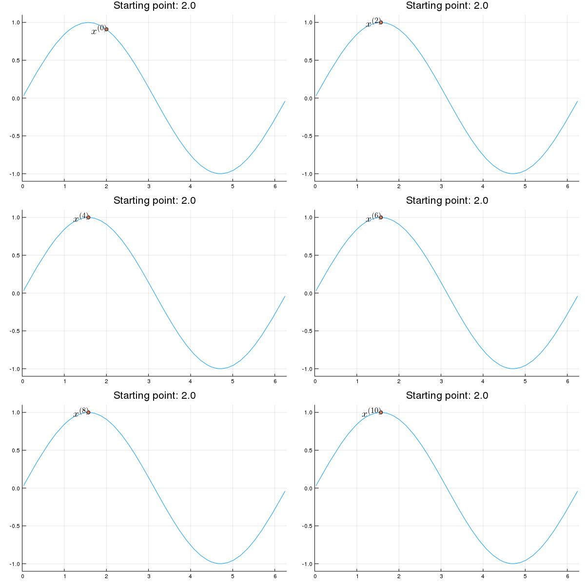
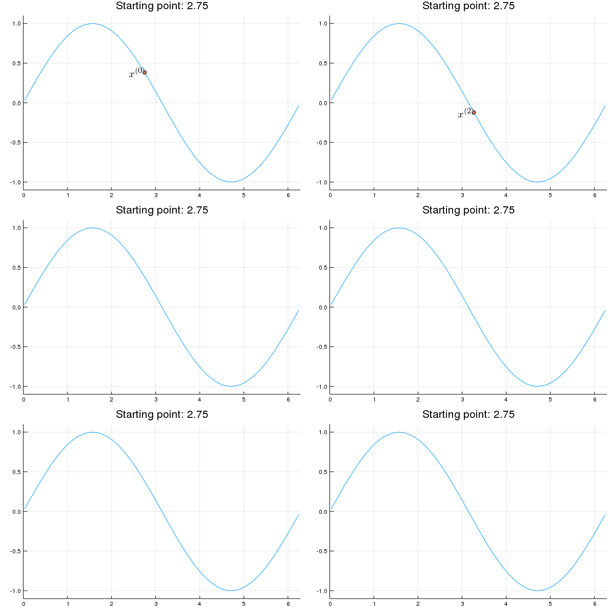
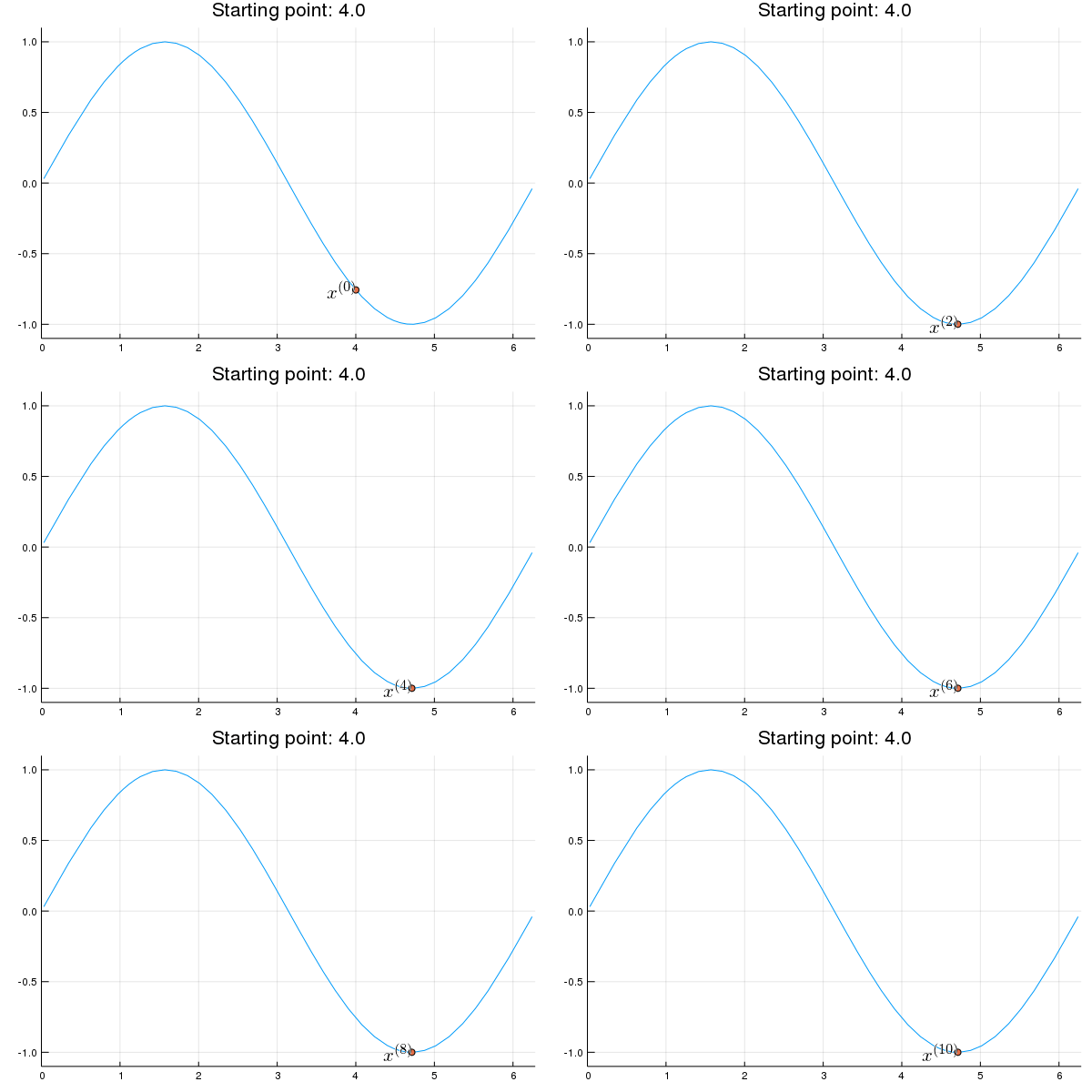
Stability issue: naive Newton's iterate is not guaranteed to be an ascent algorithm. It's equally happy to head uphill or downhill. Following example shows that the Newton iterate converges to a local maximum, converges to a local minimum, or diverges depending on starting points.
using Plots; gr()
using LaTeXStrings, ForwardDiff

f(x) = sin(x)
df = x -> ForwardDiff.derivative(f, x) # gradient
d2f = x -> ForwardDiff.derivative(df, x) # hessian
x = 2.0 # start point: 2.0 (local maximum), 2.75 (diverge), 4.0 (local minimum)
titletext = "Starting point: $x"
anim = @animate for iter in 0:10
    iter > 0 && (global x = x - d2f(x) \ df(x))
    p = Plots.plot(f, 0, 2π, xlim=(0, 2π), ylim=(-1.1, 1.1), legend=nothing, title=titletext)
    Plots.plot!(p, [x], [f(x)], shape=:circle)
    Plots.annotate!(p, x, f(x), text(latexstring("x^{($iter)}"), :right))
end
gif(anim, "./tmp.gif", fps = 1);


Remedies for the instability issue:
- approximate $-\nabla^2L(\theta^{(t)})$ by a positive definite $\mathbf{A}$ (if it's not), and
- line search (backtracking).
Why insist on a positive definite approximation of Hessian? By first-order Taylor expansion, $$ \begin{eqnarray*} & & L(\theta^{(t)} + s \Delta \theta^{(t)}) - L(\theta^{(t)}) \\ &=& \nabla L(\theta^{(t)})^T s \Delta \theta^{(t)} + o(s) \\ &=& s \cdot \nabla L(\theta^{(t)})^T [\mathbf{A}^{(t)}]^{-1} \nabla L(\theta^{(t)}) + o(s). \end{eqnarray*} $$ For $s$ sufficiently small, right hand side is strictly positive when $\mathbf{A}^{(t)}$ is positive definite. The quantity $\{\nabla L(\theta^{(t)})^T [\mathbf{A}^{(t)}]^{-1} \nabla L(\theta^{(t)})\}^{1/2}$ is termed the Newton decrement.
In summary, a practical Newton-type algorithm iterates according to $$ \boxed{ \theta^{(t+1)} = \theta^{(t)} + s [\mathbf{A}^{(t)}]^{-1} \nabla L(\theta^{(t)}) = \theta^{(t)} + s \Delta \theta^{(t)} } $$ where $\mathbf{A}^{(t)}$ is a pd approximation of $-\nabla^2L(\theta^{(t)})$ and $s$ is a step length.
For strictly concave $L$, $-\nabla^2L(\theta^{(t)})$ is always positive definite. Line search is still needed to guarantee convergence.
Line search strategy: step-halving ($s=1,1/2,\ldots$), golden section search, cubic interpolation, Amijo rule, ... Note the Newton direction
$$ \Delta \theta^{(t)} = [\mathbf{A}^{(t)}]^{-1} \nabla L(\theta^{(t)}) $$ only needs to be calculated once. Cost of line search mainly lies in objective function evaluation.How to approximate $-\nabla^2L(\theta)$? More of an art than science. Often requires problem specific analysis.
Taking $\mathbf{A} = \mathbf{I}$ leads to the method of steepest ascent, aka gradient ascent.

Fisher's scoring method
Fisher's scoring method: replace $- \nabla^2L(\theta)$ by the expected Fisher information matrix $$ \mathbf{FIM}(\theta) = \mathbf{E}[-\nabla^2L(\theta)] = \mathbf{E}[\nabla L(\theta) \nabla L(\theta)^T] \succeq \mathbf{0}_{p \times p}, $$ which is psd under exchangeability of expectation and differentiation.
Therefore the Fisher's scoring algorithm iterates according to $$ \boxed{ \theta^{(t+1)} = \theta^{(t)} + s [\mathbf{FIM}(\theta^{(t)})]^{-1} \nabla L(\theta^{(t)})}. $$
Generalized linear model (GLM) (KL 14.7)
Logistic regression
Let's consider a concrete example: logistic regression.
The goal is to predict whether a credit card transaction is fraud ($y_i=1$) or not ($y_i=0$). Predictors ($\mathbf{x}_i$) include: time of transaction, last location, merchant, ...
$y_i \in \{0,1\}$, $\mathbf{x}_i \in \mathbb{R}^{p}$. Model $y_i \sim $Bernoulli$(p_i)$.
Logistic regression. Density $$ \begin{eqnarray*} f(y_i|p_i) &=& p_i^{y_i} (1-p_i)^{1-y_i} \\ &=& e^{y_i \ln p_i + (1-y_i) \ln (1-p_i)} \\ &=& e^{y_i \ln \frac{p_i}{1-p_i} + \ln (1-p_i)}, \end{eqnarray*} $$ where $$ \begin{eqnarray*} \mathbf{E} (y_i) = p_i &=& \frac{e^{\eta_i}}{1+ e^{\eta_i}} \quad \text{(mean function, inverse link function)} \\ \eta_i = \mathbf{x}_i^T \beta &=& \ln \left( \frac{p_i}{1-p_i} \right) \quad \text{(logit link function)}. \end{eqnarray*} $$
Given data $(y_i,\mathbf{x}_i)$, $i=1,\ldots,n$,
- Newton's method == Fisher's scoring iteration: $$ \begin{eqnarray*} \beta^{(t+1)} &=& \beta^{(t)} + s[-\nabla^2 L(\beta^{(t)})]^{-1} \nabla L(\beta^{(t)}) \\ &=& \beta^{(t)} + s(\mathbf{X}^T \mathbf{W}^{(t)} \mathbf{X})^{-1} \mathbf{X}^T (\mathbf{y} - \mathbf{p}^{(t)}) \\ &=& (\mathbf{X}^T \mathbf{W}^{(t)} \mathbf{X})^{-1} \mathbf{X}^T \mathbf{W}^{(t)} \left[ \mathbf{X} \beta^{(t)} + s(\mathbf{W}^{(t)})^{-1} (\mathbf{y} - \mathbf{p}^{(t)}) \right] \\ &=& (\mathbf{X}^T \mathbf{W}^{(t)} \mathbf{X})^{-1} \mathbf{X}^T \mathbf{W}^{(t)} \mathbf{z}^{(t)}, \end{eqnarray*} $$ where $$ \mathbf{z}^{(t)} = \mathbf{X} \beta^{(t)} + s(\mathbf{W}^{(t)})^{-1} (\mathbf{y} - \mathbf{p}^{(t)}) $$ are the working responses. A Newton's iteration is equivalent to solving a weighed least squares problem $\sum_{i=1}^n w_i (z_i - \mathbf{x}_i^T \beta)^2$. Thus the name IRWLS (iteratively re-weighted least squares).
GLM
Let's consider the more general class of generalized linear models (GLM).
| Family | Canonical Link | Variance Function |
|---|---|---|
| Normal | $\eta=\mu$ | 1 |
| Poisson | $\eta=\log \mu$ | $\mu$ |
| Binomial | $\eta=\log \left( \frac{\mu}{1 - \mu} \right)$ | $\mu (1 - \mu)$ |
| Gamma | $\eta = \mu^{-1}$ | $\mu^2$ |
| Inverse Gaussian | $\eta = \mu^{-2}$ | $\mu^3$ |
$Y$ belongs to an exponential family with density $$ p(y|\theta,\phi) = \exp \left\{ \frac{y\theta - b(\theta)}{a(\phi)} + c(y,\phi) \right\}. $$
- $\theta$: natural parameter.
- $\phi>0$: dispersion parameter.
GLM relates the mean $\mu = \mathbf{E}(Y|\mathbf{x})$ via a strictly increasing link function $$ g(\mu) = \eta = \mathbf{x}^T \beta, \quad \mu = g^{-1}(\eta) $$
Score, Hessian, information
Fisher scoring method $$ \beta^{(t+1)} = \beta^{(t)} + s [\mathbf{FIM}(\beta^{(t)})]^{-1} \nabla L_n(\beta^{(t)}) $$ IRWLS with weights $w_i = [\mu_i(\eta_i)]^2/\sigma_i^2$ and some working responses $z_i$.
For canonical link, $\theta = \eta$, the second term of Hessian vanishes and Hessian coincides with Fisher information matrix. Convex problem 😄 $$ \text{Fisher's scoring == Newton's method}. $$
Non-canonical link, non-convex problem 😞 $$ \text{Fisher's scoring algorithm} \ne \text{Newton's method}. $$ Example: Probit regression (binary response with probit link). $$ \begin{eqnarray*} y_i &\sim& \text{Bernoulli}(p_i) \\ p_i &=& \Phi(\mathbf{x}_i^T \beta) \\ \eta_i &=& \mathbf{x}_i^T \beta = \Phi^{-1}(p_i). \end{eqnarray*} $$ where $\Phi(\cdot)$ is the cdf of a standard normal.
Julia, R and Matlab implement the Fisher scoring method, aka IRWLS, for GLMs.
- GLM.jl package.
Nonlinear regression - Gauss-Newton method (KL 14.4-14.6)
Now we finally get to the problem Gauss faced in 1800!
Relocate Ceres by fitting 41 observations to a 6-parameter (nonlinear) orbit.Nonlinear least squares (curve fitting): $$ \text{minimize} \,\, f(\beta) = \frac{1}{2} \sum_{i=1}^n [y_i - \mu_i(\mathbf{x}_i, \beta)]^2 $$ For example, $y_i =$ dry weight of onion and $x_i=$ growth time, and we want to fit a 3-parameter growth curve $$ \mu(x, \beta_1,\beta_2,\beta_3) = \frac{\beta_3}{1 + e^{-\beta_1 - \beta_2 x}}. $$

"Score" and "information matrices" $$ \begin{eqnarray*} \nabla f(\beta) &=& - \sum_{i=1}^n [y_i - \mu_i(\beta)] \nabla \mu_i(\beta) \\ \nabla^2 f(\beta) &=& \sum_{i=1}^n \nabla \mu_i(\beta) \nabla \mu_i(\beta)^T - \sum_{i=1}^n [y_i - \mu_i(\beta)] \nabla^2 \mu_i(\beta) \\ \mathbf{FIM}(\beta) &=& \sum_{i=1}^n \nabla \mu_i(\beta) \nabla \mu_i(\beta)^T = \mathbf{J}(\beta)^T \mathbf{J}(\beta), \end{eqnarray*} $$ where $\mathbf{J}(\beta)^T = [\nabla \mu_1(\beta), \ldots, \nabla \mu_n(\beta)] \in \mathbb{R}^{p \times n}$.
Gauss-Newton (= "Fisher's scoring algorithm") uses $\mathbf{I}(\beta)$, which is always psd. $$ \boxed{ \beta^{(t+1)} = \beta^{(t)} + s [\mathbf{FIM} (\beta^{(t)})]^{-1} \nabla L(\beta^{(t)}) } $$
Levenberg-Marquardt method, aka damped least squares algorithm (DLS), adds a ridge term to the approximate Hessian $$ \boxed{ \beta^{(t+1)} = \beta^{(t)} + s [\mathbf{FIM} (\beta^{(t)}) + \tau \mathbf{I}_p]^{-1} \nabla L(\beta^{(t)}) } $$ bridging between Gauss-Newton and steepest descent.
Other approximation to Hessians: nonlinear GLMs.
See KL 14.4 for examples.