Table of Contents¶

Paper	Citations (5/20/2019)	Per Year
Kaplan-Meier (Kaplan and Meier, 1958)	55672	913
EM algorithm (Dempster et al., 1977)	55195	1314
FDR (Benjamini and Hochberg, 1995)	54787	2283
Cox model (Cox, 1972)	49275	1048
Metropolis algorithm (Metropolis et al., 1953)	39181	594
lasso (Tibshrani, 1996)	28074	1221
Unit root test (Dickey and Fuller, 1979)	24947	624
bootstrap (Efron, 1979)	17626	441
FFT (Cooley and Tukey, 1965)	14635	271
Gibbs sampler (Gelfand and Smith, 1990)	7884	272

Citation counts from Google Scholar on May 20, 2019.
EM is one of the most influential statistical ideas, finding applications in various branches of science.
History: Landmark paper Dempster et al., 1977 on EM algorithm. Same idea appears in parameter estimation in HMM (Baum-Welch algorithm) by Baum et al., 1970.

EM algorithm¶

Goal: maximize the log-likelihood of the observed data $\ln g(\mathbf{y}|\theta)$ (optimization!)
Notations:
- $\mathbf{Y}$: observed data
- $\mathbf{Z}$: missing data
Idea: choose missing $\mathbf{Z}$ such that MLE for the complete data is easy.
Let $f(\mathbf{y},\mathbf{z} | \theta)$ be the density of complete data.
Iterative two-step procedure
- E step: calculate the conditional expectation $$ Q(\theta|\theta^{(t)}) = \mathbf{E}_{\mathbf{Z}|\mathbf{Y}=\mathbf{y},\theta^{(t)}} [ \ln f(\mathbf{Y},\mathbf{Z}|\theta) \mid \mathbf{Y} = \mathbf{y}, \theta^{(t)}] $$
- M step: maximize $Q(\theta|\theta^{(t)})$ to generate the next iterate $$ \theta^{(t+1)} = \text{argmax}_{\theta} \, Q(\theta|\theta^{(t)}) $$
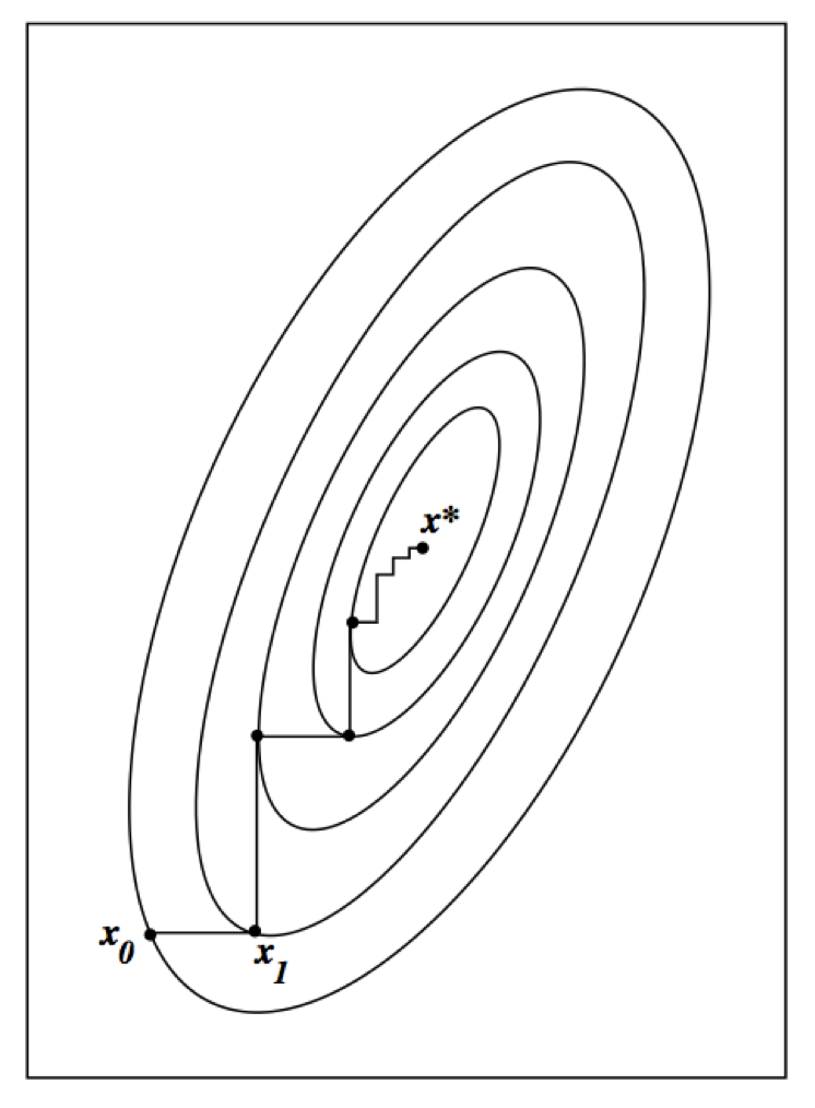
(Ascent property of EM algorithm) By the information inequality, $$ \begin{eqnarray*} & & Q(\theta \mid \theta^{(t)}) - \ln g(\mathbf{y}|\theta) \\ &=& \mathbf{E} [\ln f(\mathbf{Y},\mathbf{Z}|\theta) | \mathbf{Y} = \mathbf{y}, \theta^{(t)}] - \ln g(\mathbf{y}|\theta) \\ &=& \mathbf{E} \left\{ \ln \left[ \frac{f(\mathbf{Y}, \mathbf{Z} \mid \theta)}{g(\mathbf{Y} \mid \theta)} \right] \mid \mathbf{Y} = \mathbf{y}, \theta^{(t)} \right\} \\ &\le& \mathbf{E} \left\{ \ln \left[ \frac{f(\mathbf{Y}, \mathbf{Z} \mid \theta^{(t)})}{g(\mathbf{Y} \mid \theta^{(t)})} \right] \mid \mathbf{Y} = \mathbf{y}, \theta^{(t)} \right\} \\ &=& Q(\theta^{(t)} \mid \theta^{(t)}) - \ln g(\mathbf{y} |\theta^{(t)}). \end{eqnarray*} $$ Rearranging shows that (fundamental inequality of EM) $$ \begin{eqnarray*} \ln g(\mathbf{y} \mid \theta) \ge Q(\theta \mid \theta^{(t)}) - Q(\theta^{(t)} \mid \theta^{(t)}) + \ln g(\mathbf{y} \mid \theta^{(t)}) \end{eqnarray*} $$ for all $\theta$; in particular $$ \begin{eqnarray*} \ln g(\mathbf{y} \mid \theta^{(t+1)}) &\ge& Q(\theta^{(t+1)} \mid \theta^{(t)}) - Q(\theta^{(t)} \mid \theta^{(t)}) + \ln g(\mathbf{y} \mid \theta^{(t)}) \\ &\ge& \ln g(\mathbf{y} \mid \theta^{(t)}). \end{eqnarray*} $$ Obviously we only need $$ Q(\theta^{(t+1)} \mid \theta^{(t)}) - Q(\theta^{(t)} \mid \theta^{(t)}) \ge 0 $$ for this ascent property to hold (generalized EM).
Intuition? Keep these pictures in mind

Under mild conditions, $\theta^{(t)}$ converges to a stationary point of $\ln g(\mathbf{y} \mid \theta)$.
Numerous applications of EM:
finite mixture model, HMM (Baum-Welch algorithm), factor analysis, variance components model aka linear mixed model (LMM), hyper-parameter estimation in empirical Bayes procedure $\max_{\alpha} \int f(\mathbf{y}|\theta) \pi(\theta|\alpha) \, d \theta$, missing data, group/censorized/truncated model, ...

See Chapters 13 of Numerical Analysis for Statisticians by Kenneth Lange (2010) for more applications of EM.

A canonical EM example: finite mixture models¶

Consider Gaussian finite mixture models with density $$ h(\mathbf{y}) = \sum_{j=1}^k \pi_j h_j(\mathbf{y} \mid \mu_j, \Omega_j), \quad \mathbf{y} \in \mathbf{R}^{d}, $$ where $$ h_j(\mathbf{y} \mid \mu_j, \Omega_j) = \left( \frac{1}{2\pi} \right)^{d/2} \det(\Omega_j)^{-1/2} e^{- \frac 12 (\mathbf{y} - \mu_j)^T \Omega_j^{-1} (\mathbf{y} - \mu_j)} $$ are densities of multivariate normals $N_d(\mu_j, \Omega_j)$.
Given iid data points $\mathbf{y}_1,\ldots,\mathbf{y}_n$, want to estimate parameters $$ \theta = (\pi_1, \ldots, \pi_k, \mu_1, \ldots, \mu_k, \Omega_1,\ldots,\Omega_k) $$ subject to constraint $\pi_j \ge 0, \sum_{j=1}^d \pi_j = 1, \Omega_j \succeq \mathbf{0}$.
(Incomplete) data log-likelihood is \begin{eqnarray*} \ln g(\mathbf{y}_1,\ldots,\mathbf{y}_n|\theta) &=& \sum_{i=1}^n \ln h(\mathbf{y}_i) = \sum_{i=1}^n \ln \sum_{j=1}^k \pi_j h_j(\mathbf{y}_i \mid \mu_j, \Omega_j) \\ &=& \sum_{i=1}^n \ln \left[ \sum_{j=1}^k \pi_j \left( \frac{1}{2\pi} \right)^{d/2} \det(\Omega_j)^{-1/2} e^{- \frac 12 (\mathbf{y}_i - \mu_j)^T \Omega_j^{-1} (\mathbf{y}_i - \mu_j)} \right]. \end{eqnarray*}
Let $z_{ij} = I \{\mathbf{y}_i$ comes from group $j \}$ be the missing data. The complete data likelihood is $$ \begin{eqnarray*} f(\mathbf{y},\mathbf{z} | \theta) = \prod_{i=1}^n \prod_{j=1}^k [\pi_j h_j(\mathbf{y}_i|\mu_j,\Omega_j)]^{z_{ij}} \end{eqnarray*} $$ and thus the complete log-likelihood is $$ \begin{eqnarray*} \ln f(\mathbf{y},\mathbf{z} | \theta) = \sum_{i=1}^n \sum_{j=1}^k z_{ij} [\ln \pi_j + \ln h_j(\mathbf{y}_i|\mu_j,\Omega_j)]. \end{eqnarray*} $$
E step: need to evaluate conditional expectation $$ \begin{eqnarray*} & & Q(\theta|\theta^{(t)}) = \mathbf{E} \left\{ \sum_{i=1}^n \sum_{j=1}^k z_{ij} [\ln \pi_j + \ln h_j(\mathbf{y}_i|\mu_j,\Omega_j)] \mid \mathbf{Y}=\mathbf{y}, \pi^{(t)}, \mu_1^{(t)}, \ldots, \mu_k^{(t)}, \Omega_1^{(t)}, \ldots, \Omega_k^{(t)} ] \right\}. \end{eqnarray*} $$ By Bayes rule, we have $$ \begin{eqnarray*} w_{ij}^{(t)} &:=& \mathbf{E} [z_{ij} \mid \mathbf{y}, \pi^{(t)}, \mu_1^{(t)}, \ldots, \mu_k^{(t)}, \Omega_1^{(t)}, \ldots, \Omega_k^{(t)}] \\ &=& \frac{\pi_j^{(t)} h_j(\mathbf{y}_i|\mu_j^{(t)},\Omega_j^{(t)})}{\sum_{j'=1}^k \pi_{j'}^{(t)} h_{j'}(\mathbf{y}_i|\mu_{j'}^{(t)},\Omega_{j'}^{(t)})}. \end{eqnarray*} $$ So the Q function becomes $$ \begin{eqnarray*} & & Q(\theta|\theta^{(t)}) = \sum_{i=1}^n \sum_{j=1}^k w_{ij}^{(t)} \ln \pi_j + \sum_{i=1}^n \sum_{j=1}^k w_{ij}^{(t)} \left[ - \frac{1}{2} \ln \det \Omega_j - \frac{1}{2} (\mathbf{y}_i - \mu_j)^T \Omega_j^{-1} (\mathbf{y}_i - \mu_j) \right]. \end{eqnarray*} $$
M step: maximizer of the Q function gives the next iterate $$ \begin{eqnarray*} \pi_j^{(t+1)} &=& \frac{\sum_i w_{ij}^{(t)}}{n} \\ \mu_j^{(t+1)} &=& \frac{\sum_{i=1}^n w_{ij}^{(t)} \mathbf{y}_i}{\sum_{i=1}^n w_{ij}^{(t)}} \\ \Omega_j^{(t+1)} &=& \frac{\sum_{i=1}^n w_{ij}^{(t)} (\mathbf{y}_i - \mu_j^{(t+1)}) (\mathbf{y}_i - \mu_j^{(t+1)})^T}{\sum_i w_{ij}^{(t)}}. \end{eqnarray*} $$ See KL Example 11.3.1 for multinomial MLE. See KL Example 11.2.3 for multivariate normal MLE.
Compare these extremely simple updates to Newton type algorithms!
Also note the ease of parallel computing with this EM algorithm. See, e.g.,
Suchard, M. A.; Wang, Q.; Chan, C.; Frelinger, J.; Cron, A.; West, M. Understanding GPU programming for statistical computation: studies in massively parallel massive mixtures. Journal of Computational and Graphical Statistics, 2010, 19, 419-438.

Generalizations of EM - handle difficulties in M step¶

Expectation Conditional Maximization (ECM)¶

Meng and Rubin (1993).
In some problems the M step is difficult (no analytic solution).
Conditional maximization is easy (block ascent).
- partition parameter vector into blocks $\theta = (\theta_1, \ldots, \theta_B)$.
- alternately update $\theta_b$, $b=1,\ldots,B$.

Ascent property still holds. Why?
ECM may converge slower than EM (more iterations) but the total computer time may be shorter due to ease of the CM step.

ECM Either (ECME)¶

Liu and Rubin (1994).
Each CM step maximizes either the $Q$ function or the original incomplete observed log-likelihood.
Ascent property still holds. Why?
Faster convergence than ECM.

Alternating ECM (AECM)¶

Meng and van Dyk (1997).
The specification of the complete-data is allowed to be different on each CM-step.
Ascent property still holds. Why?

PX-EM and efficient data augmentation¶

Parameter-Expanded EM. Liu, Rubin, and Wu (1998), Liu and Wu (1999).
Efficient data augmentation. Meng and van Dyk (1997).
Idea: Speed up the convergence of EM algorithm by efficiently augmenting the observed data (introducing a working parameter in the specification of complete data).

Example: t distribution¶

EM¶

$\mathbf{W} \in \mathbb{R}^{p}$ is a multivariate $t$-distribution $t_p(\mu,\Sigma,\nu)$ if $\mathbf{W} \sim N(\mu, \Sigma/u)$ and $u \sim \text{gamma}\left(\frac{\nu}{2}, \frac{\nu}{2}\right)$.
Widely used for robust modeling.
Recall Gamma($\alpha,\beta$) has density \begin{eqnarray*} f(u \mid \alpha,\beta) = \frac{\beta^{\alpha} u^{\alpha-1}}{\Gamma(\alpha)} e^{-\beta u}, \quad u \ge 0, \end{eqnarray*} with mean $\mathbf{E}(U)=\alpha/\beta$, and $\mathbf{E}(\log U) = \psi(\alpha) - \log \beta$.
Density of $\mathbf{W}$ is \begin{eqnarray*} f_p(\mathbf{w} \mid \mu, \Sigma, \nu) = \frac{\Gamma \left(\frac{\nu+p}{2}\right) \text{det}(\Sigma)^{-1/2}}{(\pi \nu)^{p/2} \Gamma(\nu/2) [1 + \delta (\mathbf{w},\mu;\Sigma)/\nu]^{(\nu+p)/2}}, \end{eqnarray*} where \begin{eqnarray*} \delta (\mathbf{w},\mu;\Sigma) = (\mathbf{w} - \mu)^T \Sigma^{-1} (\mathbf{w} - \mu) \end{eqnarray*} is the Mahalanobis squared distance between $\mathbf{w}$ and $\mu$.
Given iid data $\mathbf{w}_1, \ldots, \mathbf{w}_n$, the log-likelihood is \begin{eqnarray*} L(\mu, \Sigma, \nu) &=& - \frac{np}{2} \log (\pi \nu) + n \left[ \log \Gamma \left(\frac{\nu+p}{2}\right) - \log \Gamma \left(\frac{\nu}{2}\right) \right] \\ && - \frac n2 \log \det \Sigma + \frac n2 (\nu + p) \log \nu \\ && - \frac{\nu + p}{2} \sum_{j=1}^n \log [\nu + \delta (\mathbf{w}_j,\mu;\Sigma) ] \end{eqnarray*} How to compute the MLE $(\hat \mu, \hat \Sigma, \hat \nu)$?
$\mathbf{W}_j | u_j$ independent $N(\mu,\Sigma/u_j)$ and $U_j$ iid gamma $\left(\frac{\nu}{2},\frac{\nu}{2}\right)$.
Missing data: $\mathbf{z}=(u_1,\ldots,u_n)^T$.
Log-likelihood of complete data is \begin{eqnarray*} L_c (\mu, \Sigma, \nu) &=& - \frac{np}{2} \ln (2\pi) - \frac{n}{2} \log \det \Sigma \\ & & - \frac 12 \sum_{j=1}^n u_j (\mathbf{w}_j - \mu)^T \Sigma^{-1} (\mathbf{w}_j - \mu) \\ & & - n \log \Gamma \left(\frac{\nu}{2}\right) + \frac{n \nu}{2} \log \left(\frac{\nu}{2}\right) \\ & & + \frac{\nu}{2} \sum_{j=1}^n (\log u_j - u_j) - \sum_{j=1}^n \log u_j. \end{eqnarray*}
Since gamma is the conjugate prior for normal-gamma model, conditional distribution of $U$ given $\mathbf{W} = \mathbf{w}$ is gamma$((\nu+p)/2, (\nu + \delta(\mathbf{w},\mu; \Sigma))/2)$. Thus \begin{eqnarray*} \mathbf{E} (U_j \mid \mathbf{w}_j, \mu^{(t)},\Sigma^{(t)},\nu^{(t)}) &=& \frac{\nu^{(t)} + p}{\nu^{(t)} + \delta(\mathbf{w}_j,\mu^{(t)};\Sigma^{(t)})} =: u_j^{(t)} \\ \mathbf{E} (\log U_j \mid \mathbf{w}_j, \mu^{(t)},\Sigma^{(t)},\nu^{(t)}) &=& \log u_j^{(t)} + \left[ \psi \left(\frac{\nu^{(t)}+p}{2}\right) - \log \left(\frac{\nu^{(t)}+p}{2}\right) \right]. \end{eqnarray*}
Overall $Q$ function (up to an additive constant) takes the form \begin{eqnarray*} %Q(\mubf,\Sigmabf,\nu \mid \mubf^{(t)},\Sigmabf^{(t)},\nu^{(t)}) = & & - \frac n2 \log \det \Sigma - \frac 12 \sum_{j=1}^n u_j^{(t)} (\mathbf{w}_j - \mu)^T \Sigma^{-1} (\mathbf{w}_j - \mu) \\ & & - n \log \Gamma \left(\frac{\nu}{2}\right) + \frac{n \nu}{2} \log \left(\frac{\nu}{2}\right) \\ & & + \frac{n \nu}{2} \left[ \frac 1n \sum_{j=1}^n \left(\log u_j^{(t)} - u_j^{(t)}\right) + \psi\left(\frac{\nu^{(t)}+p}{2}\right) - \log \left(\frac{\nu^{(t)}+p}{2}\right) \right]. \end{eqnarray*}
Maximization over $(\mu, \Sigma)$ is simply a weighted multivariate normal problem \begin{eqnarray*} \mu^{(t+1)} &=& \frac{\sum_{j=1}^n u_j^{(t)} \mathbf{w}_j}{\sum_{j=1}^n u_j^{(t)}} \\ \Sigma^{(t+1)} &=& \frac 1n \sum_{j=1}^n u_j^{(t)} (\mathbf{w}_j - \mu^{(t+1)}) (\mathbf{w}_j - \mu^{(t+1)})^T. \end{eqnarray*} Notice down-weighting of outliers is obvious in the update.
Maximization over $\nu$ is a univariate problem - Brent method, golden section, or bisection.

ECM and ECME¶

Partition parameter $(\mu,\Sigma,\nu)$ into two blocks $(\mu,\Sigma)$ and $\nu$:

ECM = EM for this example. Why?
ECME: In the second CM step, maximize over $\nu$ in terms of the original log-likelihood function instead of the $Q$ function. They have similar difficulty since both are univariate optimization problems!
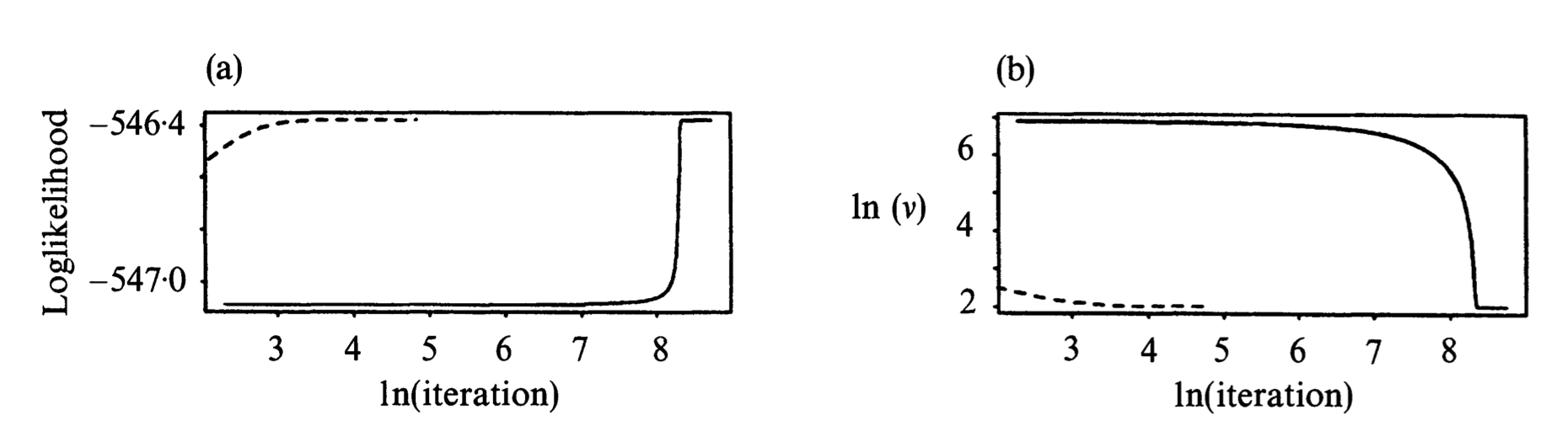
An example from Liu and Rubin (1994). $n=79$, $p=2$, with missing entries. EM=ECM: solid line. ECME: dashed line.

Efficient data augmentation¶

Assume $\nu$ known:

Write $\mathbf{W}_j = \mu + \mathbf{C}_j / U_j^{1/2}$, where $\mathbf{C}_j$ is $N(\mathbf{0},\Sigma)$ independent of $U_j$ which is gamma$\left(\frac{\nu}{2},\frac{\nu}{2}\right)$.
$\mathbf{W}_j = \mu + \det (\Sigma)^{-a/2} \mathbf{C}_j / U_j^{1/2}(a)$, where $U_j(a) = \det(\Sigma)^{-a} U_j$.
Then the complete data is $(\mathbf{w}, \mathbf{z}(a))$, $a$ the working parameter.
$a=0$ corresponds to the vanilla EM.
Meng and van Dyk (1997) recommend using $a_{\text{opt}} = 1/(\nu+p)$ to maximize the convergence rate.
Exercise: work out the EM update for this special case.
The only change to the vanilla EM is to replace the denominator $n$ in the update of $\Sigma$ by $\sum_{j=1}^n u_j^{(t)}$.
PX-EM (Liu, Rubin, and Wu, 1998) leads to the same update.

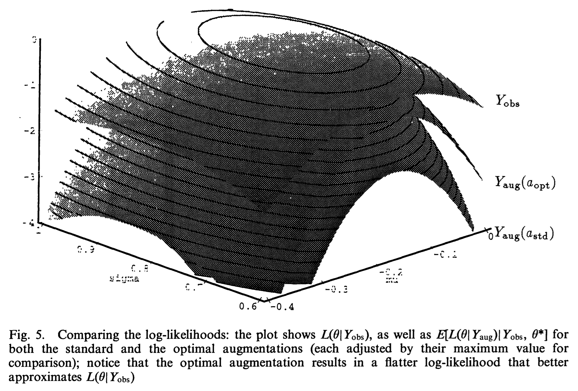
Assume $\nu$ unknown:

Version 1: $a=a_{\text{opt}}$ in both updating of $(\mu,\Sigma)$ and $\nu$.
Version 2: $a=a_{\text{opt}}$ for updating $(\mu,\Sigma)$ and taking the observed data as complete data for updating $\nu$.

Conclusion in Meng and van Dyk (1997): Version 1 is $8 \sim 12$ faster than EM=ECM or ECME. Version 2 is only slightly more efficient than Version 1

Generalizations of EM - handle difficulties in E step¶

Monte Carlo EM (MCEM)¶

Wei and Tanner (1990).
Hard to calculate $Q$ function? Simulate! \begin{eqnarray*} Q(\theta \mid \theta^{(t)}) \approx \frac 1m \sum_{j=1}^m \ln f(\mathbf{y}, \mathbf{z}_j \mid \theta), \end{eqnarray*} where $\mathbf{z}_j$ are iid from conditional distribution of missing data given $\mathbf{y}$ and previous iterate $\theta^{(t)}$.
Ascent property may be lost due to Monte Carlo errors.
Example: capture-recapture model, generalized linear mixed model (GLMM).

Stochastic EM (SEM) and Simulated Annealing EM (SAEM)¶

SEM

Celeux and Diebolt (1985).
Same as MCEM with $m=1$. A single draw of missing data $\mathbf{z}$ from the conditional distribution.
$\theta^{(t)}$ forms a Markov chain which converges to a stationary distribution. No definite relation between this stationary distribution and the MLE.
In some specific cases, it can be shown that the stationary distribution concentrates around the MLE with a variance inversely proportional to the sample size.
Advantage: can escape the attraction to inferior mode/saddle point in some mixture model problems.

SAEM

Celeux and Deibolt (1989).
Increase $m$ with the iterations, ending up with an EM algorithm.

Data-augmentation (DA) algorithm¶

Tanner and Wong (1987).
Aim for sampling from $p(\theta|\mathbf{y})$ instead of maximization.
Idea: incomplete data posterior density is complicated, but the complete-data posterior density is relatively easy to sample.
Data augmentation algorithm:
- draw $\mathbf{z}^{(t+1)}$ conditional on $(\theta^{(t)},\mathbf{y})$
- draw $\theta^{(t+1)}$ conditional on $(\mathbf{z}^{(t+1)},\mathbf{y})$
A special case of Gibbs sampler.
$\theta^{(t)}$ converges to the distribution $p(\theta|\mathbf{y})$ under general conditions.
Ergodic mean converges to the posterior mean $\mathbf{E}(\theta|\mathbf{y})$, which may perform better than MLE in finite sample.

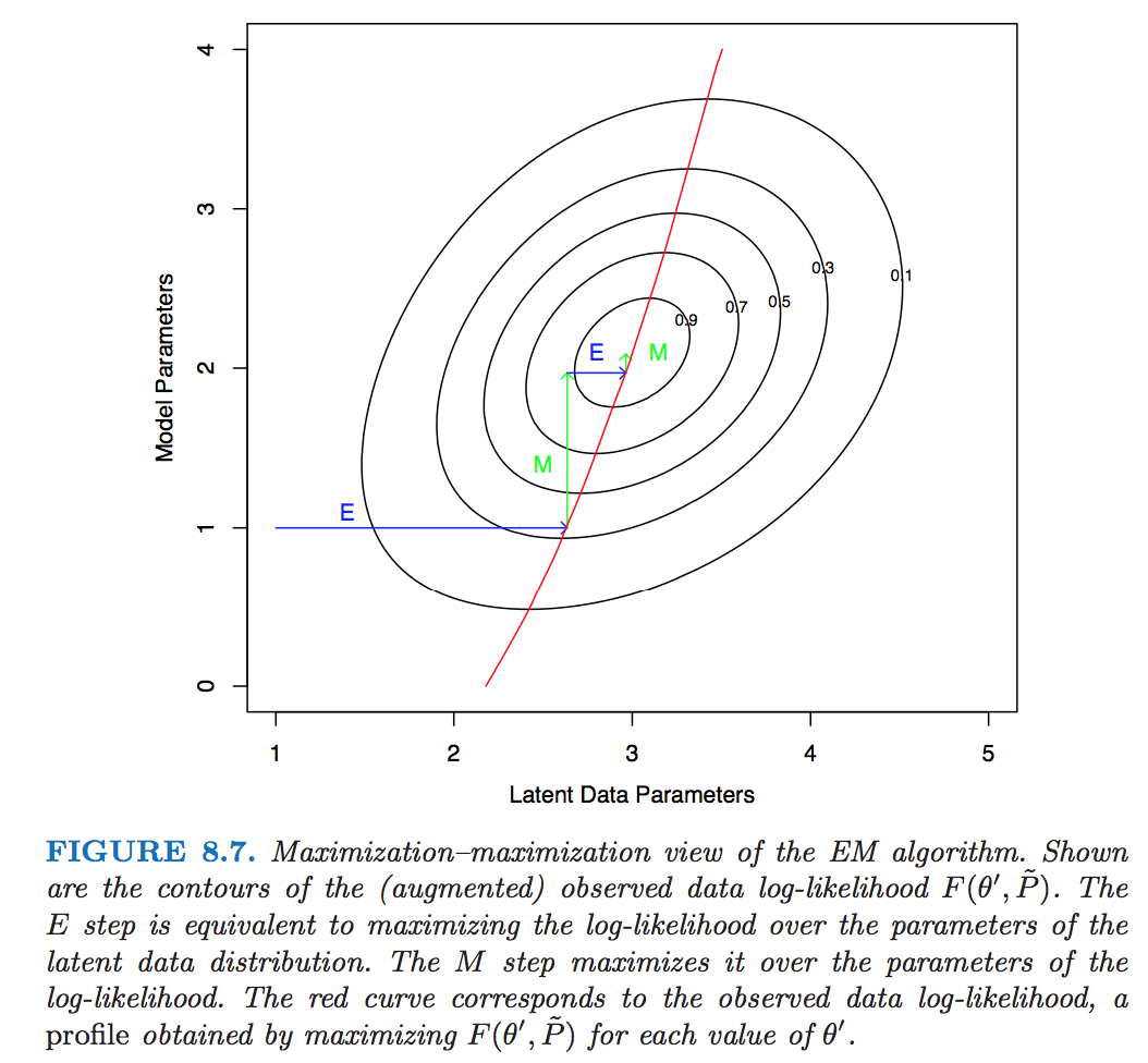
EM as a maximization-maximization procedure¶

Neal and Hinton (1999).
Consider the objective function \begin{eqnarray*} F(\theta, q) = \mathbf{E}_q [\ln f(\mathbf{Z},\mathbf{y} \mid \theta)] + H(q) \end{eqnarray*} over $\Theta \times {\cal Q}$, where ${\cal Q}$ is the set of all conditional pdfs of the missing data $\{q(\mathbf{z}) = p(\mathbf{z} \mid \mathbf{y}, \theta), \theta \in \Theta \}$ and $H(q) = -\mathbf{E}_q \log q$ is the entropy of $q$.
EM is essentially performing coordinate ascent for maximizing $F$
- E step: At current iterate $\theta^{(t)}$,
  \begin{eqnarray*} F(\theta^{(t)}, q) = \mathbf{E}_q [\log p(\mathbf{Z} \mid \mathbf{y}, \theta^{(t)})] - \mathbf{E}_q \log q + \ln g(\mathbf{y} \mid \theta^{(t)}). \end{eqnarray*} The maximizing conditional pdf is given by $q = \log f(\mathbf{Z} \mid \mathbf{y}, \theta^{(t)})$
- M step: Substitute $q = \log f(\mathbf{Z} \mid \mathbf{y}, \theta^{(t)})$ into $F$ and maximize over $\theta$

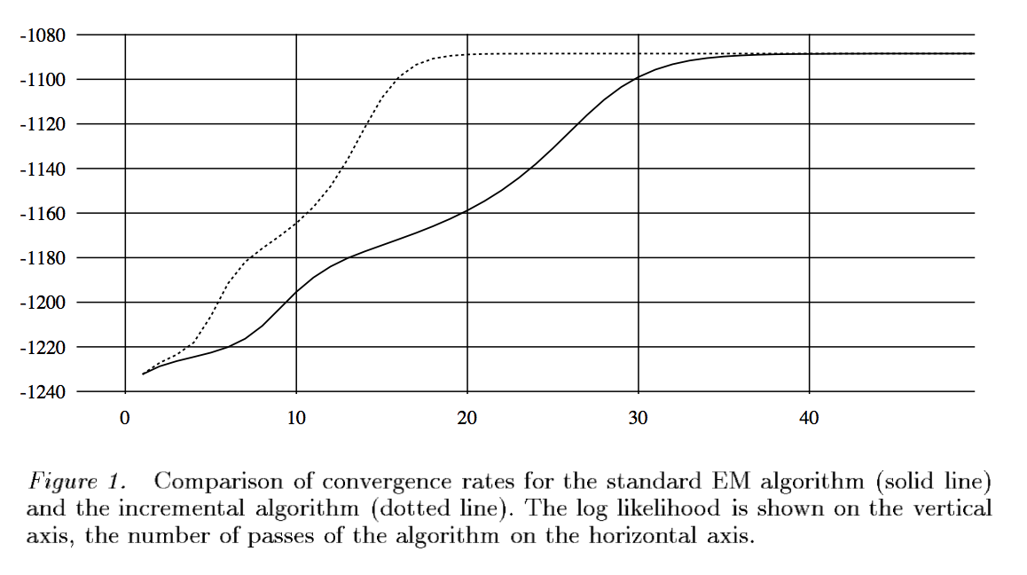
Incremental EM¶

Assume iid observations. Then the objective function is \begin{eqnarray*} F(\theta,q) = \sum_i \left[ \mathbf{E}_{q_i} \log p(\mathbf{Z}_i,\mathbf{y}_i \mid \theta) + H(q_i) \right], \end{eqnarray*} where we search for $q$ under factored form $q(\mathbf{z}) = \prod_i q_i (\mathbf{z})$.
Maximizing $F$ over $q$ is equivalent to maximizing the contribution of each data with respect to $q_i$.
Update $\theta$ by visiting data items sequentially rather than from a global E step.
Finite mixture example: for each data point $i$
- evaluate membership variables $w_{ij}$, $j=1,\ldots,k$.
- update parameter values $(\pi^{(t+1)}, \mu_j^{(t+1)}, \Sigma_j^{(t+1)})$ (only need to keep sufficient statistics!)
Faster convergence than vanilla EM in some examples.