Numerical linear algebra

System information (for reproducibility)

In [1]:
versioninfo()
Julia Version 1.7.3
Commit 742b9abb4d (2022-05-06 12:58 UTC)
Platform Info:
  OS: macOS (x86_64-apple-darwin21.4.0)
  CPU: Intel(R) Core(TM) i7-6920HQ CPU @ 2.90GHz
  WORD_SIZE: 64
  LIBM: libopenlibm
  LLVM: libLLVM-12.0.1 (ORCJIT, skylake)
Environment:
  JULIA_EDITOR = code
  JULIA_NUM_THREADS = 4

Introduction

  • Topics in numerical algebra:

    • BLAS
    • solve linear equations $\mathbf{A} \mathbf{x} = \mathbf{b}$
    • regression computations $\mathbf{X}^T \mathbf{X} \beta = \mathbf{X}^T \mathbf{y}$
    • eigen-problems $\mathbf{A} \mathbf{x} = \lambda \mathbf{x}$
    • generalized eigen-problems $\mathbf{A} \mathbf{x} = \lambda \mathbf{B} \mathbf{x}$
    • singular value decompositions $\mathbf{A} = \mathbf{U} \Sigma \mathbf{V}^T$
    • iterative methods for numerical linear algebra
  • Except for the iterative methods, most of these numerical linear algebra tasks are implemented in the BLAS and LAPACK libraries. They form the building blocks of most statistical computing tasks (optimization, MCMC).

  • All high-level languages (R, Matlab, Julia) call BLAS and LAPACK for numerical linear algebra.

    • Julia offers more flexibility by exposing interfaces to many BLAS/LAPACK subroutines directly. See documentation.

BLAS

  • BLAS stands for basic linear algebra subprograms.

  • See netlib for a complete list of standardized BLAS functions.

  • There are many implementations of BLAS.

    • Netlib provides a reference implementation.
    • Matlab uses Intel's MKL (mathematical kernel libaries). MKL implementation is the gold standard on market. It is not open source but the compiled library is free for Linux and MacOS.
    • Julia uses OpenBLAS. OpenBLAS is the best open source implementation.
  • There are 3 levels of BLAS functions.

Level Example Operation Name Dimension Flops
1 $\alpha \gets \mathbf{x}^T \mathbf{y}$ dot product $\mathbf{x}, \mathbf{y} \in \mathbb{R}^n$ $2n$
1 $\mathbf{y} \gets \mathbf{y} + \alpha \mathbf{x}$ axpy $\alpha \in \mathbb{R}$, $\mathbf{x}, \mathbf{y} \in \mathbb{R}^n$ $2n$
2 $\mathbf{y} \gets \mathbf{y} + \mathbf{A} \mathbf{x}$ gaxpy $\mathbf{A} \in \mathbb{R}^{m \times n}$, $\mathbf{x} \in \mathbb{R}^n$, $\mathbf{y} \in \mathbb{R}^m$ $2mn$
2 $\mathbf{A} \gets \mathbf{A} + \mathbf{y} \mathbf{x}^T$ rank one update $\mathbf{A} \in \mathbb{R}^{m \times n}$, $\mathbf{x} \in \mathbb{R}^n$, $\mathbf{y} \in \mathbb{R}^m$ $2mn$
3 $\mathbf{C} \gets \mathbf{C} + \mathbf{A} \mathbf{B}$ matrix multiplication $\mathbf{A} \in \mathbb{R}^{m \times p}$, $\mathbf{B} \in \mathbb{R}^{p \times n}$, $\mathbf{C} \in \mathbb{R}^{m \times n}$ $2mnp$
  • Typical BLAS functions support single precision (S), double precision (D), complex (C), and double complex (Z).

Examples

The form of a mathematical expression and the way the expression should be evaluated in actual practice may be quite different.

Some operations appear as level-3 but indeed are level-2.

Example 1. A common operation in statistics is column scaling or row scaling $$ \begin{eqnarray*} \mathbf{A} &=& \mathbf{A} \mathbf{D} \quad \text{(column scaling)} \\ \mathbf{A} &=& \mathbf{D} \mathbf{A} \quad \text{(row scaling)}, \end{eqnarray*} $$ where $\mathbf{D}$ is diagonal. For example, in generalized linear models (GLMs), the Fisher information matrix takes the form
$$ \mathbf{X}^T \mathbf{W} \mathbf{X}, $$ where $\mathbf{W}$ is a diagonal matrix with observation weights on diagonal.

Column and row scalings are essentially level-2 operations!

In [2]:
using BenchmarkTools, LinearAlgebra, Random

Random.seed!(123) # seed
n = 2000
A = rand(n, n) # n-by-n matrix
d = rand(n)  # n vector
D = Diagonal(d) # diagonal matrix with d as diagonal
Out[2]:
2000×2000 Diagonal{Float64, Vector{Float64}}:
 0.919181   ⋅         ⋅         ⋅        …   ⋅         ⋅          ⋅ 
  ⋅        0.426019   ⋅         ⋅            ⋅         ⋅          ⋅ 
  ⋅         ⋅        0.746586   ⋅            ⋅         ⋅          ⋅ 
  ⋅         ⋅         ⋅        0.819201      ⋅         ⋅          ⋅ 
  ⋅         ⋅         ⋅         ⋅            ⋅         ⋅          ⋅ 
  ⋅         ⋅         ⋅         ⋅        …   ⋅         ⋅          ⋅ 
  ⋅         ⋅         ⋅         ⋅            ⋅         ⋅          ⋅ 
  ⋅         ⋅         ⋅         ⋅            ⋅         ⋅          ⋅ 
  ⋅         ⋅         ⋅         ⋅            ⋅         ⋅          ⋅ 
  ⋅         ⋅         ⋅         ⋅            ⋅         ⋅          ⋅ 
  ⋅         ⋅         ⋅         ⋅        …   ⋅         ⋅          ⋅ 
  ⋅         ⋅         ⋅         ⋅            ⋅         ⋅          ⋅ 
  ⋅         ⋅         ⋅         ⋅            ⋅         ⋅          ⋅ 
 ⋮                                       ⋱                       
  ⋅         ⋅         ⋅         ⋅            ⋅         ⋅          ⋅ 
  ⋅         ⋅         ⋅         ⋅            ⋅         ⋅          ⋅ 
  ⋅         ⋅         ⋅         ⋅        …   ⋅         ⋅          ⋅ 
  ⋅         ⋅         ⋅         ⋅            ⋅         ⋅          ⋅ 
  ⋅         ⋅         ⋅         ⋅            ⋅         ⋅          ⋅ 
  ⋅         ⋅         ⋅         ⋅            ⋅         ⋅          ⋅ 
  ⋅         ⋅         ⋅         ⋅            ⋅         ⋅          ⋅ 
  ⋅         ⋅         ⋅         ⋅        …   ⋅         ⋅          ⋅ 
  ⋅         ⋅         ⋅         ⋅            ⋅         ⋅          ⋅ 
  ⋅         ⋅         ⋅         ⋅           0.572021   ⋅          ⋅ 
  ⋅         ⋅         ⋅         ⋅            ⋅        0.0403848   ⋅ 
  ⋅         ⋅         ⋅         ⋅            ⋅         ⋅         0.141618
In [3]:
Dfull = convert(Matrix, D) # convert to full matrix
Out[3]:
2000×2000 Matrix{Float64}:
 0.919181  0.0       0.0       0.0       …  0.0       0.0        0.0
 0.0       0.426019  0.0       0.0          0.0       0.0        0.0
 0.0       0.0       0.746586  0.0          0.0       0.0        0.0
 0.0       0.0       0.0       0.819201     0.0       0.0        0.0
 0.0       0.0       0.0       0.0          0.0       0.0        0.0
 0.0       0.0       0.0       0.0       …  0.0       0.0        0.0
 0.0       0.0       0.0       0.0          0.0       0.0        0.0
 0.0       0.0       0.0       0.0          0.0       0.0        0.0
 0.0       0.0       0.0       0.0          0.0       0.0        0.0
 0.0       0.0       0.0       0.0          0.0       0.0        0.0
 0.0       0.0       0.0       0.0       …  0.0       0.0        0.0
 0.0       0.0       0.0       0.0          0.0       0.0        0.0
 0.0       0.0       0.0       0.0          0.0       0.0        0.0
 ⋮                                       ⋱                       
 0.0       0.0       0.0       0.0          0.0       0.0        0.0
 0.0       0.0       0.0       0.0          0.0       0.0        0.0
 0.0       0.0       0.0       0.0       …  0.0       0.0        0.0
 0.0       0.0       0.0       0.0          0.0       0.0        0.0
 0.0       0.0       0.0       0.0          0.0       0.0        0.0
 0.0       0.0       0.0       0.0          0.0       0.0        0.0
 0.0       0.0       0.0       0.0          0.0       0.0        0.0
 0.0       0.0       0.0       0.0       …  0.0       0.0        0.0
 0.0       0.0       0.0       0.0          0.0       0.0        0.0
 0.0       0.0       0.0       0.0          0.572021  0.0        0.0
 0.0       0.0       0.0       0.0          0.0       0.0403848  0.0
 0.0       0.0       0.0       0.0          0.0       0.0        0.141618
In [4]:
# this is calling BLAS routine for matrix multiplication: O(n^3) flops
# this is SLOW!
@benchmark $A * $Dfull
Out[4]:
BenchmarkTools.Trial: 42 samples with 1 evaluation.
 Range (minmax):   97.589 ms202.120 ms   GC (min … max): 0.00% … 0.15%
 Time  (median):     116.057 ms                GC (median):    0.00%
 Time  (mean ± σ):   121.254 ms ±  21.703 ms   GC (mean ± σ):  1.77% ± 2.70%

   ▁▄ █▁   ▁█ ▄▁ ▁▄                    ▄                         
  ▆██▆██▆▆▆██████▆▆▆▁▁▆▁▁▁▁▁▁▁▁▁▁▁▁▁▁█▁▁▁▁▆▁▁▁▁▁▁▁▁▁▁▁▁▁▁▁▁▁▆ ▁
  97.6 ms          Histogram: frequency by time          202 ms <

 Memory estimate: 30.52 MiB, allocs estimate: 2.
In [5]:
# dispatch to special method for diagonal matrix multiplication.
# columnwise scaling: O(n^2) flops
@benchmark $A * $D
Out[5]:
BenchmarkTools.Trial: 426 samples with 1 evaluation.
 Range (minmax):   9.075 ms19.795 ms   GC (min … max):  0.00% … 42.32%
 Time  (median):      9.685 ms               GC (median):     0.00%
 Time  (mean ± σ):   11.717 ms ±  3.066 ms   GC (mean ± σ):  18.21% ± 18.97%

   █▆▅                           ▅▅▂▁▂▁          
  ▇████▇▅█▅▆▁▅▆▅▅▁▁▄▁▄▁▁▁▁▁▁▁▁▁▁▁▁▁▁▁▁▁▁▄▁▁▁▆██████▅▄▅▁▅▄▄▄ ▇
  9.08 ms      Histogram: log(frequency) by time      17.6 ms <

 Memory estimate: 30.52 MiB, allocs estimate: 4.
In [6]:
# in-place: avoid allocate space for result
# rmul!: compute matrix-matrix product AB, overwriting A, and return the result.
@benchmark rmul!($A, $D)
Out[6]:
BenchmarkTools.Trial: 429 samples with 1 evaluation.
 Range (minmax):   5.184 ms21.888 ms   GC (min … max): 0.00% … 0.00%
 Time  (median):     11.604 ms               GC (median):    0.00%
 Time  (mean ± σ):   11.679 ms ±  4.733 ms   GC (mean ± σ):  0.00% ± 0.00%

    ██▆█▃▃ ▁         ▅      ▄▁  ▃     ▁           ▁           
  ▆▆██████▇█▇▆▁▃▁▃▃▃▅█▆▃▇▄█▇██▆▇█▄▄▃▆▆█▆▃▄▇▅▄▃▃▃▄▇█▄▄▃▃▃█▃▅▃ ▄
  5.18 ms         Histogram: frequency by time        21.5 ms <

 Memory estimate: 96 bytes, allocs estimate: 2.

Note: In R or Matlab, diag(d) will create a full matrix. Be cautious using diag function: do we really need a full diagonal matrix?

In [7]:
using RCall

R"""
d <- runif(5)
diag(d)
"""
Out[7]:
RObject{RealSxp}
          [,1]      [,2]      [,3]      [,4]       [,5]
[1,] 0.3830245 0.0000000 0.0000000 0.0000000 0.00000000
[2,] 0.0000000 0.5793777 0.0000000 0.0000000 0.00000000
[3,] 0.0000000 0.0000000 0.2344167 0.0000000 0.00000000
[4,] 0.0000000 0.0000000 0.0000000 0.4607606 0.00000000
[5,] 0.0000000 0.0000000 0.0000000 0.0000000 0.01739585

Example 2. Innter product between two matrices $\mathbf{A}, \mathbf{B} \in \mathbb{R}^{m \times n}$ is often written as $$ \text{trace}(\mathbf{A}^T \mathbf{B}), \text{trace}(\mathbf{B} \mathbf{A}^T), \text{trace}(\mathbf{A} \mathbf{B}^T), \text{ or } \text{trace}(\mathbf{B}^T \mathbf{A}). $$ They appear as level-3 operation (matrix multiplication with $O(m^2n)$ or $O(mn^2)$ flops).

In [8]:
Random.seed!(123)
n = 2000
A, B = randn(n, n), randn(n, n)

# slow way to evaluate this thing
@benchmark tr(transpose($A) * $B)
Out[8]:
BenchmarkTools.Trial: 36 samples with 1 evaluation.
 Range (minmax):  117.910 ms172.937 ms   GC (min … max): 0.00% … 0.00%
 Time  (median):     138.821 ms                GC (median):    0.00%
 Time  (mean ± σ):   140.982 ms ±  14.105 ms   GC (mean ± σ):  1.78% ± 2.50%

           █▃          ▃     ▃        ▃    █ ▃                ▃  
  ▇▁▁▁▇▁▇▇▁██▁▁▇▇▁▇▇▇▁▇█▇▇▇█▁▁▇▁▁▇▁▁█▇▁▁▁█▁█▁▁▁▁▁▁▁▇▁▁▁▁▁▁▁▁█ ▁
  118 ms           Histogram: frequency by time          173 ms <

 Memory estimate: 30.52 MiB, allocs estimate: 2.

But $\text{trace}(\mathbf{A}^T \mathbf{B}) = <\text{vec}(\mathbf{A}), \text{vec}(\mathbf{B})>$. The latter is level-2 operation with $O(mn)$ flops.

In [9]:
@benchmark dot($A, $B)
Out[9]:
BenchmarkTools.Trial: 1330 samples with 1 evaluation.
 Range (minmax):  2.419 ms 31.788 ms   GC (min … max): 0.00% … 0.00%
 Time  (median):     3.662 ms                GC (median):    0.00%
 Time  (mean ± σ):   3.727 ms ± 993.942 μs   GC (mean ± σ):  0.00% ± 0.00%

                    ▁▂▃▄▂▆▄▅▄▆▅▃▂▂   ▁                      
  ▃▂▁▂▂▁▂▁▂▂▂▃▃▃▄▄▆▇██████████████▇▇██▆▅▄▃▄▃▄▄▂▃▃▂▃▂▁▂▂▂▁▂ ▄
  2.42 ms         Histogram: frequency by time        5.02 ms <

 Memory estimate: 0 bytes, allocs estimate: 0.

Example 3. Similarly $\text{diag}(\mathbf{A}^T \mathbf{B})$ can be calculated in $O(mn)$ flops.

In [10]:
# slow way to evaluate this thing: O(n^3)
@benchmark diag(transpose($A) * $B)
Out[10]:
BenchmarkTools.Trial: 39 samples with 1 evaluation.
 Range (minmax):  107.914 ms186.092 ms   GC (min … max): 0.00% … 5.03%
 Time  (median):     130.929 ms                GC (median):    0.00%
 Time  (mean ± σ):   130.798 ms ±  16.272 ms   GC (mean ± σ):  1.95% ± 2.72%

   ▃█   ▃   █        █    ▃▃   █   ▃                            
  ▇██▁▇▇█▇▁▇█▁▁▇▁▇▇▁█▇▁▇▇██▁▇▁█▇▁▁█▁▁▁▁▁▁▁▁▁▁▁▁▁▁▁▁▁▁▁▁▁▁▁▁▁▇ ▁
  108 ms           Histogram: frequency by time          186 ms <

 Memory estimate: 30.53 MiB, allocs estimate: 3.
In [11]:
# smarter: O(n^2)
@benchmark Diagonal(vec(sum($A .* $B, dims=1)))
Out[11]:
BenchmarkTools.Trial: 459 samples with 1 evaluation.
 Range (minmax):   8.016 ms18.824 ms   GC (min … max):  0.00% … 39.49%
 Time  (median):      9.045 ms               GC (median):     0.00%
 Time  (mean ± σ):   10.880 ms ±  3.106 ms   GC (mean ± σ):  19.35% ± 19.71%

  ▃█    ▇                                                      
  ████▇▇█▆▄▃▂▂▂▃▂▂▂▂▁▁▁▁▁▁▁▁▁▁▂▁▁▁▁▁▁▃▅▆▅▅▄▂▄▃▂▂▃▇▃▅▃▄▁▃▂▁▂ ▃
  8.02 ms         Histogram: frequency by time        17.2 ms <

 Memory estimate: 30.53 MiB, allocs estimate: 5.

To get rid of allocation of intermediate array at all, we can just write a double loop or use dot function.

In [12]:
using LoopVectorization

function diag_matmul!(d, A, B)
    m, n = size(A)
    @assert size(B) == (m, n) "A and B should have same size"
    fill!(d, 0)
    @avx for j in 1:n, i in 1:m
        d[j] += A[i, j] * B[i, j]
    end
#     for j in 1:n
#         @views d[j] = dot(A[:, j], B[:, j])
#     end
    Diagonal(d)
end

d = zeros(eltype(A), size(A, 2))
@benchmark diag_matmul!($d, $A, $B)
┌ Info: Precompiling LoopVectorization [bdcacae8-1622-11e9-2a5c-532679323890]
└ @ Base loading.jl:1423
Out[12]:
BenchmarkTools.Trial: 1113 samples with 1 evaluation.
 Range (minmax):  3.406 ms  7.880 ms   GC (min … max): 0.00% … 0.00%
 Time  (median):     4.288 ms                GC (median):    0.00%
 Time  (mean ± σ):   4.468 ms ± 797.065 μs   GC (mean ± σ):  0.00% ± 0.00%

    ▁▅█▃▅▆▂▂             ▂                                     
  ▄▄█████████▆▇▆▆▆▅▆▆▇██▇█▆▇▄▄▆▆▅▅▄▄▃▃▄▃▅▅▄▄▅▄▃▄▃▃▃▃▃▃▁▃▁▃▂ ▄
  3.41 ms         Histogram: frequency by time         6.6 ms <

 Memory estimate: 0 bytes, allocs estimate: 0.

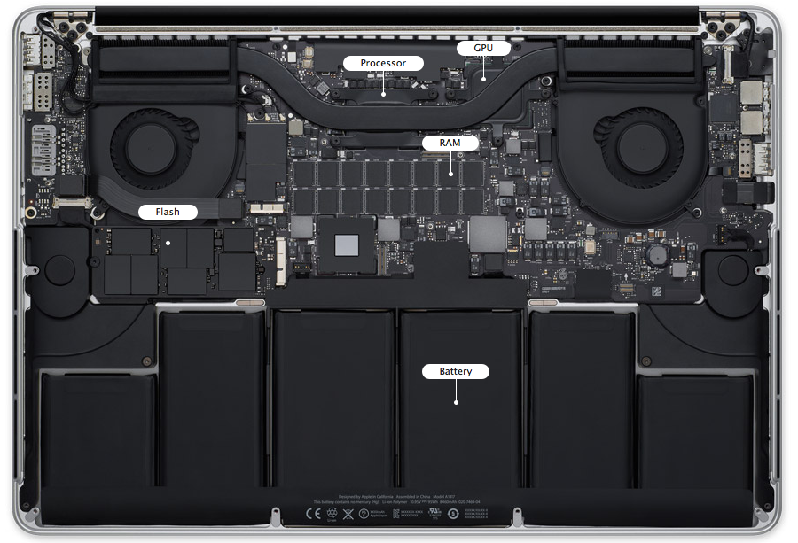
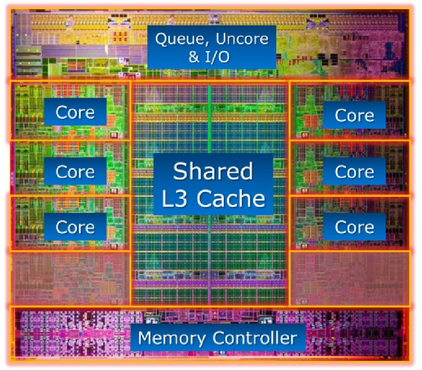
Memory hierarchy and level-3 fraction

Key to high performance is effective use of memory hierarchy. True on all architectures.

  • Flop count is not the sole determinant of algorithm efficiency. Another important factor is data movement through the memory hierarchy.

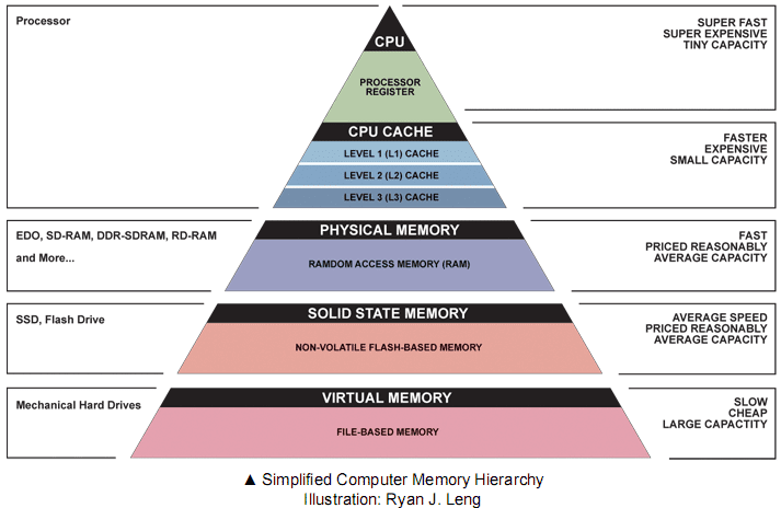
  • Numbers everyone should know
Operation Time
L1 cache reference 0.5 ns
L2 cache reference 7 ns
Main memory reference 100 ns
Read 1 MB sequentially from memory 250,000 ns
Read 1 MB sequentially from SSD 1,000,000 ns
Read 1 MB sequentially from disk 20,000,000 ns

Source: https://gist.github.com/jboner/2841832

  • For example, Xeon X5650 CPU has a theoretical throughput of 128 DP GFLOPS but a max memory bandwidth of 32GB/s.

  • Can we keep CPU cores busy with enough deliveries of matrix data and ship the results to memory fast enough to avoid backlog?
    Answer: use high-level BLAS as much as possible.

BLAS Dimension Mem. Refs. Flops Ratio
Level 1: $\mathbf{y} \gets \mathbf{y} + \alpha \mathbf{x}$ $\mathbf{x}, \mathbf{y} \in \mathbb{R}^n$ $3n$ $2n$ 3:2
Level 2: $\mathbf{y} \gets \mathbf{y} + \mathbf{A} \mathbf{x}$ $\mathbf{x}, \mathbf{y} \in \mathbb{R}^n$, $\mathbf{A} \in \mathbb{R}^{n \times n}$ $n^2$ $2n^2$ 1:2
Level 3: $\mathbf{C} \gets \mathbf{C} + \mathbf{A} \mathbf{B}$ $\mathbf{A}, \mathbf{B}, \mathbf{C} \in\mathbb{R}^{n \times n}$ $4n^2$ $2n^3$ 2:n
  • Higher level BLAS (3 or 2) make more effective use of arithmetic logic units (ALU) by keeping them busy. Surface-to-volume effect.
    See Dongarra slides.

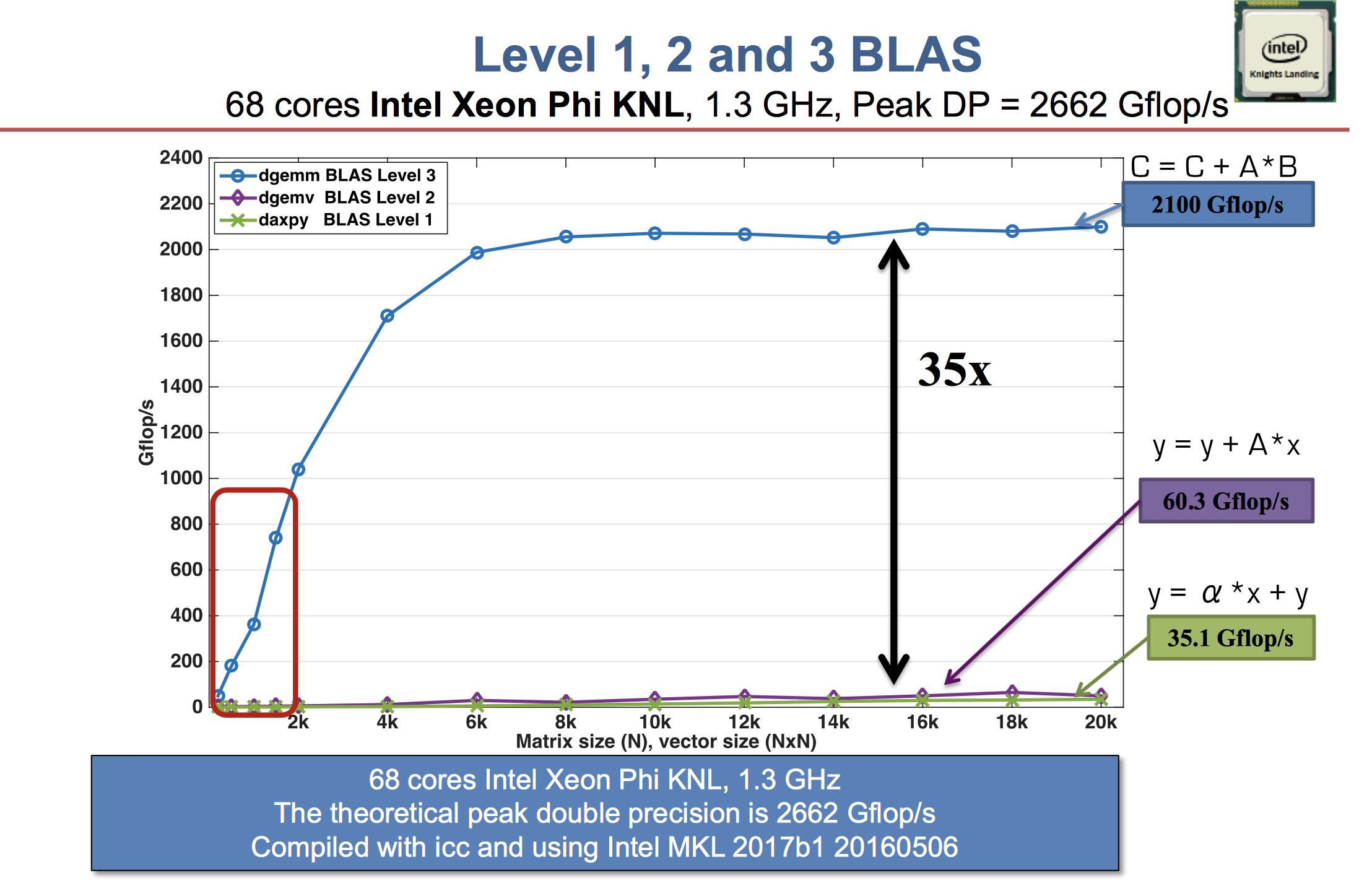
  • A distinction between LAPACK and LINPACK (older version of R uses LINPACK) is that LAPACK makes use of higher level BLAS as much as possible (usually by smart partitioning) to increase the so-called level-3 fraction.

  • To appreciate the efforts in an optimized BLAS implementation such as OpenBLAS (evolved from GotoBLAS), see the Quora question, especially the video. Bottomline is

Get familiar with (good implementations of) BLAS/LAPACK and use them as much as possible.

Effect of data layout

  • Data layout in memory affects algorithmic efficiency too. It is much faster to move chunks of data in memory than retrieving/writing scattered data.

  • Storage mode: column-major (Fortran, Matlab, R, Julia) vs row-major (C/C++).

  • Cache line is the minimum amount of cache which can be loaded and stored to memory.

    • x86 CPUs: 64 bytes
    • ARM CPUs: 32 bytes

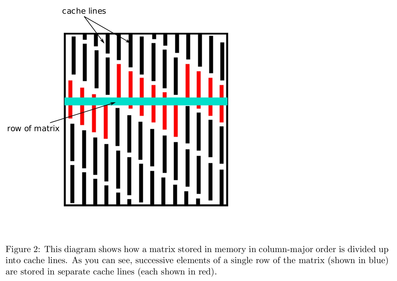
  • Accessing column-major stored matrix by rows ($ij$ looping) causes lots of cache misses.

  • Take matrix multiplication as an example $$ \mathbf{C} \gets \mathbf{C} + \mathbf{A} \mathbf{B}, \quad \mathbf{A} \in \mathbb{R}^{m \times p}, \mathbf{B} \in \mathbb{R}^{p \times n}, \mathbf{C} \in \mathbb{R}^{m \times n}. $$ Assume the storage is column-major, such as in Julia. There are 6 variants of the algorithms according to the order in the triple loops.

    • jki or kji looping:
      # inner most loop
        for i = 1:m
            C[i, j] = C[i, j] + A[i, k] * B[k, j]
        end
      
    • ikj or kij looping:
      # inner most loop        
        for j = 1:n
            C[i, j] = C[i, j] + A[i, k] * B[k, j]
        end
      
    • ijk or jik looping:
      # inner most loop        
        for k = 1:p
            C[i, j] = C[i, j] + A[i, k] * B[k, j]
        end
      
  • We pay attention to the innermost loop, where the vector calculation occurs. The associated stride when accessing the three matrices in memory (assuming column-major storage) is
Variant A Stride B Stride C Stride
$jki$ or $kji$ Unit 0 Unit
$ikj$ or $kij$ 0 Non-Unit Non-Unit
$ijk$ or $jik$ Non-Unit Unit 0

Apparently the variants $jki$ or $kji$ are preferred.

In [13]:
"""
    matmul_by_loop!(A, B, C, order)

Overwrite `C` by `A * B`. `order` indicates the looping order for triple loop.
"""
function matmul_by_loop!(A::Matrix, B::Matrix, C::Matrix, order::String)
    
    m = size(A, 1)
    p = size(A, 2)
    n = size(B, 2)
    fill!(C, 0)
    
    if order == "jki"
        @inbounds for j = 1:n, k = 1:p, i = 1:m
            C[i, j] += A[i, k] * B[k, j]
        end
    end

    if order == "kji"
        @inbounds for k = 1:p, j = 1:n, i = 1:m
            C[i, j] += A[i, k] * B[k, j]
        end
    end
    
    if order == "ikj"
        @inbounds for i = 1:m, k = 1:p, j = 1:n
            C[i, j] += A[i, k] * B[k, j]
        end
    end

    if order == "kij"
        @inbounds for k = 1:p, i = 1:m, j = 1:n
            C[i, j] += A[i, k] * B[k, j]
        end
    end
    
    if order == "ijk"
        @inbounds for i = 1:m, j = 1:n, k = 1:p
            C[i, j] += A[i, k] * B[k, j]
        end
    end
    
    if order == "jik"
        @inbounds for j = 1:n, i = 1:m, k = 1:p
            C[i, j] += A[i, k] * B[k, j]
        end
    end
    
end

using Random

Random.seed!(123)
m, p, n = 2000, 100, 2000
A = rand(m, p)
B = rand(p, n)
C = zeros(m, n);
  • $jki$ and $kji$ looping:
In [14]:
using BenchmarkTools

@benchmark matmul_by_loop!($A, $B, $C, "jki")
Out[14]:
BenchmarkTools.Trial: 68 samples with 1 evaluation.
 Range (minmax):  69.088 ms84.099 ms   GC (min … max): 0.00% … 0.00%
 Time  (median):     73.383 ms               GC (median):    0.00%
 Time  (mean ± σ):   74.120 ms ±  3.892 ms   GC (mean ± σ):  0.00% ± 0.00%

   ▅▂█▂      ▂▂▅         ▂   ▂    ▂                            
  ▅██████▁▁▅▅███▁▅▅▅▅▅▅█▅█▁█▅▅▁▅█▅▅█▅▅▁▅▁▁▅▁▁▁▅▁▁▁▅▁▁▁▁▁▅▁▅ ▁
  69.1 ms         Histogram: frequency by time          84 ms <

 Memory estimate: 0 bytes, allocs estimate: 0.
In [15]:
@benchmark matmul_by_loop!($A, $B, $C, "kji")
Out[15]:
BenchmarkTools.Trial: 12 samples with 1 evaluation.
 Range (minmax):  439.908 ms466.728 ms   GC (min … max): 0.00% … 0.00%
 Time  (median):     450.413 ms                GC (median):    0.00%
 Time  (mean ± σ):   453.000 ms ±   9.185 ms   GC (mean ± σ):  0.00% ± 0.00%

  █ █          █     █  █     █  █                  ██ █  
  █▁█▁▁▁▁▁▁▁▁▁▁█▁▁▁▁▁█▁▁██▁▁▁▁▁▁▁▁▁█▁▁█▁▁▁▁▁▁▁▁▁▁▁▁▁▁▁▁▁▁██▁█ ▁
  440 ms           Histogram: frequency by time          467 ms <

 Memory estimate: 0 bytes, allocs estimate: 0.
  • $ikj$ and $kij$ looping:
In [16]:
@benchmark matmul_by_loop!($A, $B, $C, "ikj")
Out[16]:
BenchmarkTools.Trial: 2 samples with 1 evaluation.
 Range (minmax):  2.553 s  2.570 s   GC (min … max): 0.00% … 0.00%
 Time  (median):     2.562 s               GC (median):    0.00%
 Time  (mean ± σ):   2.562 s ± 12.348 ms   GC (mean ± σ):  0.00% ± 0.00%

                              ▁▁▁▁▁▁▁▁▁▁▁▁▁▁▁▁▁▁▁▁▁▁▁▁▁▁▁▁▁▁▁▁▁▁▁▁▁▁▁▁▁▁▁▁▁▁▁▁▁▁▁▁▁▁█ ▁
  2.55 s         Histogram: frequency by time        2.57 s <

 Memory estimate: 0 bytes, allocs estimate: 0.
In [17]:
@benchmark matmul_by_loop!($A, $B, $C, "kij")
Out[17]:
BenchmarkTools.Trial: 2 samples with 1 evaluation.
 Range (minmax):  2.785 s  2.823 s   GC (min … max): 0.00% … 0.00%
 Time  (median):     2.804 s               GC (median):    0.00%
 Time  (mean ± σ):   2.804 s ± 27.003 ms   GC (mean ± σ):  0.00% ± 0.00%

                               ▁▁▁▁▁▁▁▁▁▁▁▁▁▁▁▁▁▁▁▁▁▁▁▁▁▁▁▁▁▁▁▁▁▁▁▁▁▁▁▁▁▁▁▁▁▁▁▁▁▁▁▁▁▁█ ▁
  2.79 s         Histogram: frequency by time        2.82 s <

 Memory estimate: 0 bytes, allocs estimate: 0.
  • $ijk$ and $jik$ looping:
In [18]:
@benchmark matmul_by_loop!($A, $B, $C, "ijk")
Out[18]:
BenchmarkTools.Trial: 10 samples with 1 evaluation.
 Range (minmax):  502.145 ms564.525 ms   GC (min … max): 0.00% … 0.00%
 Time  (median):     524.902 ms                GC (median):    0.00%
 Time  (mean ± σ):   527.456 ms ±  21.776 ms   GC (mean ± σ):  0.00% ± 0.00%

  ██     █ █ █                    █      ██   █               █  
  ██▁▁▁▁▁█▁█▁█▁▁▁▁▁▁▁▁▁▁▁▁▁▁▁▁▁▁█▁▁▁▁▁▁██▁▁▁█▁▁▁▁▁▁▁▁▁▁▁▁▁▁▁█ ▁
  502 ms           Histogram: frequency by time          565 ms <

 Memory estimate: 0 bytes, allocs estimate: 0.
In [19]:
@benchmark matmul_by_loop!($A, $B, $C, "ijk")
Out[19]:
BenchmarkTools.Trial: 10 samples with 1 evaluation.
 Range (minmax):  504.969 ms525.714 ms   GC (min … max): 0.00% … 0.00%
 Time  (median):     509.849 ms                GC (median):    0.00%
 Time  (mean ± σ):   512.127 ms ±   6.036 ms   GC (mean ± σ):  0.00% ± 0.00%

  ▁       ▁   █▁        ▁                ▁                  ▁  
  █▁▁▁▁▁▁▁█▁▁▁██▁▁▁▁▁▁▁▁█▁▁▁▁▁▁▁▁▁▁▁▁▁▁▁▁█▁▁▁▁▁▁▁▁▁▁▁▁▁▁▁▁▁▁█ ▁
  505 ms           Histogram: frequency by time          526 ms <

 Memory estimate: 0 bytes, allocs estimate: 0.
  • Julia wraps BLAS library for matrix multiplication. We see BLAS library wins hands down (multi-threading, Strassen algorithm, higher level-3 fraction by block outer product).
In [20]:
@benchmark mul!($C, $A, $B)
Out[20]:
BenchmarkTools.Trial: 637 samples with 1 evaluation.
 Range (minmax):  7.231 ms 12.005 ms   GC (min … max): 0.00% … 0.00%
 Time  (median):     7.430 ms                GC (median):    0.00%
 Time  (mean ± σ):   7.838 ms ± 847.058 μs   GC (mean ± σ):  0.00% ± 0.00%

  █▇▆▂▂▂▂▃▃ ▂▁▁ ▁ ▁  ▁                                        
  ████████████▁███▆██▇▆▆▅▇▇█▅▅▇▄▅▅▇▄▅▇▅▄▄▆█▄▄▇▁▅▇▄▆▄▁▇▆▄▅▁▅ █
  7.23 ms      Histogram: log(frequency) by time      10.7 ms <

 Memory estimate: 0 bytes, allocs estimate: 0.
In [21]:
# direct call of BLAS wrapper function
@benchmark LinearAlgebra.BLAS.gemm!('N', 'N', 1.0, $A, $B, 0.0, $C)
Out[21]:
BenchmarkTools.Trial: 625 samples with 1 evaluation.
 Range (minmax):  7.213 ms 11.916 ms   GC (min … max): 0.00% … 0.00%
 Time  (median):     7.524 ms                GC (median):    0.00%
 Time  (mean ± σ):   7.981 ms ± 969.501 μs   GC (mean ± σ):  0.00% ± 0.00%

  ▁▆█▇▃▃▄▂▁▁▁ ▂▁                                             
  ██████████████▇▆▇▇█▆▅▆▇▅▆▇▅▄▆▆▆▅▅█▄▆█▇▄▁▅▄▄▆▇▅▄▄▄▄▄▆▄▅▄▅▄ █
  7.21 ms      Histogram: log(frequency) by time      11.5 ms <

 Memory estimate: 0 bytes, allocs estimate: 0.

Exercise: Annotate the loop in matmul_by_loop! by @avx and benchmark again.

BLAS in R

  • Tip for R user. Standard R distribution from CRAN uses a very out-dated BLAS/LAPACK library.
In [22]:
using RCall

R"""
library(dplyr)
library(bench)
bench::mark($A %*% $B) %>%
  print(width = Inf)
""";
┌ Warning: RCall.jl: 
│ Attaching package: ‘dplyr’
│ 
│ The following objects are masked from ‘package:stats’:
│ 
│     filter, lag
│ 
│ The following objects are masked from ‘package:base’:
│ 
│     intersect, setdiff, setequal, union
│ 
└ @ RCall /Users/huazhou/.julia/packages/RCall/6kphM/src/io.jl:172
# A tibble: 1 × 13
  expression               min   median `itr/sec` mem_alloc `gc/sec` n_itr  n_gc
  <bch:expr>          <bch:tm> <bch:tm>     <dbl> <bch:byt>    <dbl> <int> <dbl>
1 `#JL`$A %*% `#JL`$B    257ms    284ms      3.52    30.5MB     3.52     2     2
  total_time result                memory             time          
    <bch:tm> <list>                <list>             <list>        
1      568ms <dbl [2,000 × 2,000]> <Rprofmem [2 × 3]> <bench_tm [2]>
  gc              
  <list>          
1 <tibble [2 × 3]>
┌ Warning: RCall.jl: Warning: Some expressions had a GC in every iteration; so filtering is disabled.
└ @ RCall /Users/huazhou/.julia/packages/RCall/6kphM/src/io.jl:172
  • Re-build R from source using OpenBLAS or MKL will immediately boost linear algebra performance in R. Google build R using MKL to get started. Similarly we can build Julia using MKL.

  • Matlab uses MKL. Usually it's very hard to beat Matlab in terms of linear algebra.

Avoid memory allocation: some examples

  1. Transposing matrix is an expensive memory operation.
    • In R, the command
      t(A) %*% x
      
      will first transpose A then perform matrix multiplication, causing unnecessary memory allocation
    • Julia is smart to avoid transposing matrix if possible.
In [23]:
using Random, LinearAlgebra, BenchmarkTools
Random.seed!(123)

n = 1000
A = rand(n, n)
x = rand(n);
In [24]:
typeof(transpose(A))
Out[24]:
Transpose{Float64, Matrix{Float64}}
In [25]:
fieldnames(typeof(transpose(A)))
Out[25]:
(:parent,)
In [26]:
# same data in tranpose(A) and original matrix A
pointer(transpose(A).parent), pointer(A)
Out[26]:
(Ptr{Float64} @0x00007fa5c7000000, Ptr{Float64} @0x00007fa5c7000000)
In [27]:
# dispatch to BLAS
# does *not* actually transpose the matrix
@benchmark transpose($A) * $x
Out[27]:
BenchmarkTools.Trial: 10000 samples with 1 evaluation.
 Range (minmax):   91.285 μs374.502 μs   GC (min … max): 0.00% … 0.00%
 Time  (median):     122.037 μs                GC (median):    0.00%
 Time  (mean ± σ):   138.212 μs ±  33.536 μs   GC (mean ± σ):  0.00% ± 0.00%

           ▁█▄                                                  
  ▁▁▁▁▁▁▂▃▅████▇▄▂▂▂▂▂▂▂▂▂▂▂▂▂▂▂▂▂▂▂▂▂▂▂▂▂▂▂▂▂▂▂▂▂▂▂▂▂▂▁▁▂▁▁▁ ▂
  91.3 μs          Histogram: frequency by time          231 μs <

 Memory estimate: 7.94 KiB, allocs estimate: 1.
In [28]:
# pre-allocate result
out = zeros(size(A, 2))
@benchmark mul!($out, transpose($A), $x)
Out[28]:
BenchmarkTools.Trial: 10000 samples with 1 evaluation.
 Range (minmax):   93.211 μs915.734 μs   GC (min … max): 0.00% … 0.00%
 Time  (median):     146.899 μs                GC (median):    0.00%
 Time  (mean ± σ):   187.108 μs ±  95.276 μs   GC (mean ± σ):  0.00% ± 0.00%

    ▆█▇▅▄▃▄▄▃▄▄▃▃▃▄▃▃▂▂▂▁▁▁▁▁▂▁▂▂▂▂▂▁▂▁▁▁▁▁▁▁▁▁▁              ▂
  ▆▇█████████████████████████████████████████████████▇▇▇▇▆▆▇▅ █
  93.2 μs       Histogram: log(frequency) by time        490 μs <

 Memory estimate: 0 bytes, allocs estimate: 0.
In [29]:
# or call BLAS wrapper directly
@benchmark LinearAlgebra.BLAS.gemv!('T', 1.0, $A, $x, 0.0, $out)
Out[29]:
BenchmarkTools.Trial: 10000 samples with 1 evaluation.
 Range (minmax):   91.027 μs417.073 μs   GC (min … max): 0.00% … 0.00%
 Time  (median):     115.689 μs                GC (median):    0.00%
 Time  (mean ± σ):   130.632 μs ±  31.795 μs   GC (mean ± σ):  0.00% ± 0.00%

        ▃▅██▄▄▄▂▁ ▁▁▁▁▂▂▂▁▁▁▂▂▂▂▁▁▁▁▁▁▁▁▁▁                    ▂
  ▄▄▆▅▆████████████████████████████████████████▇▇█▇▇▇▇▆▆▆▆▆▄▆ █
  91 μs         Histogram: log(frequency) by time        246 μs <

 Memory estimate: 0 bytes, allocs estimate: 0.
  1. Broadcasting in Julia achieves vectorized code without creating intermediate arrays.

    Suppose we want to calculate elementsize maximum of absolute values of two large arrays. In R or Matlab, the command

    max(abs(X), abs(Y))
    

    will create two intermediate arrays and then one result array.

In [30]:
using RCall
Random.seed!(123)
X, Y = rand(1000, 1000), rand(1000, 1000)

R"""
library(dplyr)
library(bench)
bench::mark(max(abs($X), abs($Y))) %>%
  print(width = Inf)
""";
# A tibble: 1 × 13
  expression                           min   median `itr/sec` mem_alloc `gc/sec`
  <bch:expr>                      <bch:tm> <bch:tm>     <dbl> <bch:byt>    <dbl>
1 max(abs(`#JL`$X), abs(`#JL`$Y))   6.23ms   6.81ms      134.    15.3MB     69.0
  n_itr  n_gc total_time result    memory             time           
  <int> <dbl>   <bch:tm> <list>    <list>             <list>         
1    35    18      261ms <dbl [1]> <Rprofmem [2 × 3]> <bench_tm [53]>
  gc               
  <list>           
1 <tibble [53 × 3]>

In Julia, dot operations are fused so no intermediate arrays are created.

In [31]:
# no intermediate arrays created, only result array created
@benchmark max.(abs.($X), abs.($Y))
Out[31]:
BenchmarkTools.Trial: 2266 samples with 1 evaluation.
 Range (minmax):  1.266 ms8.482 ms   GC (min … max):  0.00% … 74.34%
 Time  (median):     1.810 ms              GC (median):     0.00%
 Time  (mean ± σ):   2.200 ms ± 1.435 ms   GC (mean ± σ):  20.51% ± 21.67%

  ▃▃▂▇▇▅▂▁                                           ▁▁▁   ▁
  ████████▆▃▁▁▁▄▁▁▁▁▁▃▁▁▁▁▁▁▁▁▁▁▁▁▁▁▁▁▁▁▁▁▁▁▅▇█▇▆▆▆████▇█ █
  1.27 ms     Histogram: log(frequency) by time     7.36 ms <

 Memory estimate: 7.63 MiB, allocs estimate: 2.

Pre-allocating result array gets rid of memory allocation at all.

In [32]:
# no memory allocation at all!
Z = zeros(size(X)) # zero matrix of same size as X
@benchmark $Z .= max.(abs.($X), abs.($Y)) # .= (vs =) is important!
Out[32]:
BenchmarkTools.Trial: 3528 samples with 1 evaluation.
 Range (minmax):  1.158 ms  3.392 ms   GC (min … max): 0.00% … 0.00%
 Time  (median):     1.342 ms                GC (median):    0.00%
 Time  (mean ± σ):   1.405 ms ± 230.774 μs   GC (mean ± σ):  0.00% ± 0.00%

    █▅▃▄▃▂ ▁                                                   
  ▂████████████▆▆▄▅▄▄▃▃▃▃▃▂▃▂▂▃▂▂▂▂▂▂▂▂▂▁▂▂▁▁▁▂▁▁▁▁▁▁▁▁▁▁▁▁ ▃
  1.16 ms         Histogram: frequency by time        2.26 ms <

 Memory estimate: 0 bytes, allocs estimate: 0.
  1. View-1) avoids creating extra copy of matrix data.
In [33]:
Random.seed!(123)
A = randn(1000, 1000)

# sum entries in a sub-matrix
@benchmark sum($A[1:2:500, 1:2:500])
Out[33]:
BenchmarkTools.Trial: 10000 samples with 1 evaluation.
 Range (minmax):   67.632 μs  8.946 ms   GC (min … max):  0.00% … 94.81%
 Time  (median):     307.151 μs                GC (median):     0.00%
 Time  (mean ± σ):   347.393 μs ± 500.222 μs   GC (mean ± σ):  10.34% ±  7.02%

                     █▆▄▄▂▁▂▁▁                                 
  ▅▄▄▃▂▂▂▁▁▁▁▁▁▁▁▁▁▁▆██████████▇▆▆▅▄▄▄▃▃▃▃▂▂▂▂▂▂▂▂▁▁▁▁▁▁▁▁▁▁▁ ▃
  67.6 μs          Histogram: frequency by time          648 μs <

 Memory estimate: 488.36 KiB, allocs estimate: 2.
In [34]:
# view avoids creating a separate sub-matrix
@benchmark sum(@view $A[1:2:500, 1:2:500])
Out[34]:
BenchmarkTools.Trial: 7035 samples with 1 evaluation.
 Range (minmax):  628.360 μs 1.365 ms   GC (min … max): 0.00% … 0.00%
 Time  (median):     683.832 μs               GC (median):    0.00%
 Time  (mean ± σ):   707.902 μs ± 66.509 μs   GC (mean ± σ):  0.00% ± 0.00%

  ▄    ▆▁ █▁▁▇▃▂▁▂▁▁▁ ▁▁                                     ▂
  █▁▅▁▅██▆███████████████████▇▇██▇█▇█▇▇▆▆█▇▇▇▇▆▇▇▇▆▇▆▆▆▅▆▅▆▆ █
  628 μs        Histogram: log(frequency) by time       998 μs <

 Memory estimate: 0 bytes, allocs estimate: 0.

The @views macro, which can be useful in some operations.

In [35]:
@benchmark @views sum($A[1:2:500, 1:2:500])
Out[35]:
BenchmarkTools.Trial: 7070 samples with 1 evaluation.
 Range (minmax):  628.356 μs 1.556 ms   GC (min … max): 0.00% … 0.00%
 Time  (median):     682.459 μs               GC (median):    0.00%
 Time  (mean ± σ):   704.399 μs ± 60.192 μs   GC (mean ± σ):  0.00% ± 0.00%

  ▃     ▅  ▁ ▆▂▂▂▁▂▁▁▁▁  ▁                                   ▁
  █▁▄▃▃▄█▄▇███████████████████▇█▇▇█▇▇▇▇▇▇▆▆▆▇▇▇▇▇▆▇▅▆▄▅▅▄▄▅▄ █
  628 μs        Histogram: log(frequency) by time       975 μs <

 Memory estimate: 0 bytes, allocs estimate: 0.