Multinomial-logit regression and sparse regression
A demo of Multinomial-logit regression and sparse regression
Contents
Generate multinomial random vectors from covariates
clear;
% reset random seed
s = RandStream('mt19937ar','Seed',1);
RandStream.setGlobalStream(s);
% sample size
n = 200;
% # covariates
p = 15;
% # bins
d = 5;
% design matrix
X = randn(n,p);
% true regression coefficients: predictors 1, 3, and 5 have effects
B = zeros(p,d-1);
nzidx = [1 3 5];
B(nzidx,:) = ones(length(nzidx),d-1);
prob = zeros(n,d);
prob(:,d) = ones(n,1);
prob(:,1:d-1) = exp(X*B);
prob = bsxfun(@times, prob, 1./sum(prob,2));
batchsize = 25+unidrnd(25,n,1);
Y = mnrnd(batchsize,prob);

zerorows = sum(Y,2);
Y=Y(zerorows~=0, :);
X=X(zerorows~=0, :);
Fit multinomial logit regression
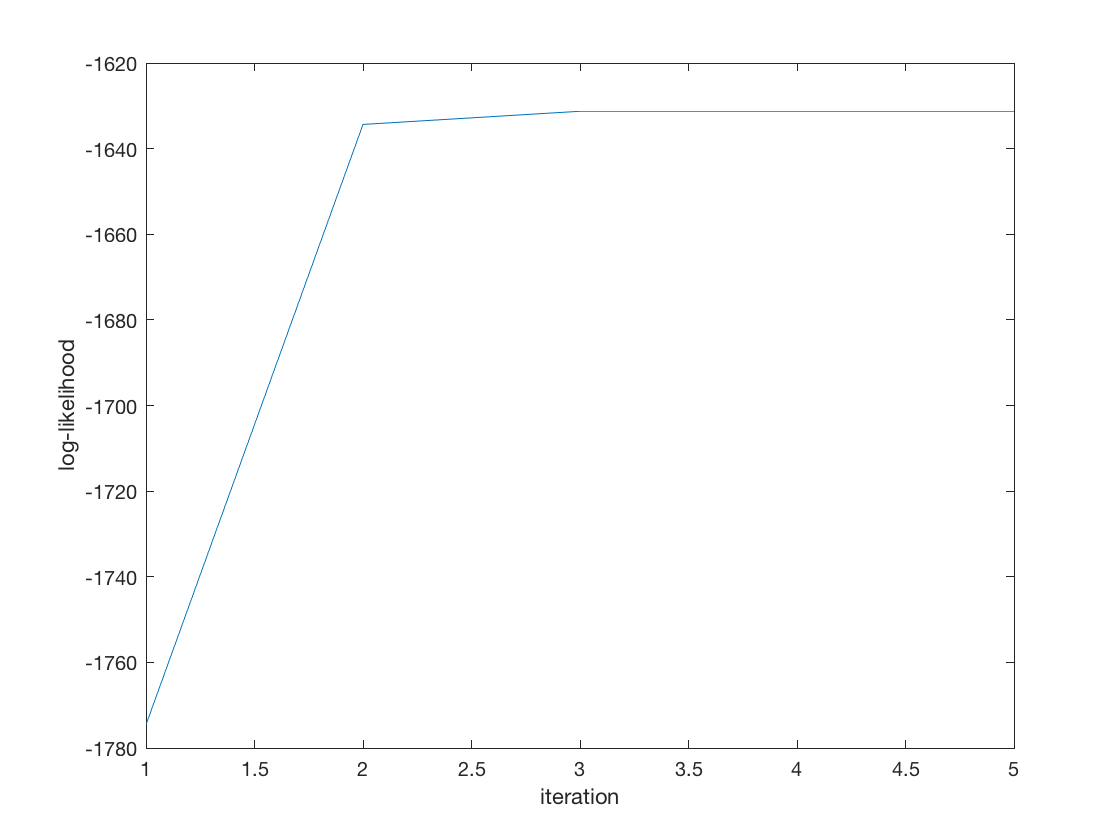
tic;
[B_hat, stats] = mnlogitreg(X,Y);
toc;
display(B_hat);
display(stats.se);
display(stats);
% Wald test of predictor significance
display('Wald test p-values:');
display(stats.wald_pvalue);

figure;
plot(stats.logL_iter);
xlabel('iteration');
ylabel('log-likelihood');
Elapsed time is 0.064823 seconds.

B_hat =

    0.9062    0.9845    0.9823    1.0066
    0.0491    0.0174    0.0223   -0.0064
    0.9543    0.9696    0.9683    0.9576
   -0.0121   -0.0053    0.0275    0.0129
    0.9871    1.0022    0.9483    0.9692
    0.0010   -0.0019   -0.0619    0.0244
   -0.0288   -0.0399   -0.0092   -0.0297
   -0.0591    0.0135   -0.0068    0.0009
   -0.0469   -0.0452   -0.0606   -0.0716
    0.0122   -0.0213   -0.0476   -0.0115
    0.0758   -0.0163    0.0003    0.0828
   -0.0039   -0.0010   -0.0128   -0.0097
   -0.0780   -0.0469   -0.0415   -0.0474
    0.0318   -0.0152   -0.0228    0.0117
   -0.0009   -0.0230   -0.0645   -0.0423

    0.0430    0.0434    0.0434    0.0436
    0.0454    0.0456    0.0455    0.0455
    0.0420    0.0421    0.0421    0.0423
    0.0415    0.0416    0.0414    0.0417
    0.0441    0.0442    0.0438    0.0441
    0.0381    0.0380    0.0380    0.0380
    0.0380    0.0382    0.0380    0.0382
    0.0387    0.0385    0.0385    0.0388
    0.0378    0.0379    0.0378    0.0380
    0.0397    0.0400    0.0401    0.0399
    0.0433    0.0433    0.0430    0.0432
    0.0427    0.0427    0.0426    0.0427
    0.0411    0.0412    0.0412    0.0413
    0.0387    0.0387    0.0387    0.0388
    0.0398    0.0398    0.0398    0.0400


stats =

  struct with fields:

                     BIC: 3.5804e+03
                     AIC: 3.3825e+03
                     dof: 60
              iterations: 5
                    logL: -1.6313e+03
               logL_iter: [1×5 double]
                    prob: [200×5 double]
                    yhat: [200×5 double]
                gradient: [60×1 double]
    observed_information: [60×60 double]
                       H: [60×60 double]
                      se: [15×4 double]
               wald_stat: [1×15 double]
             wald_pvalue: [1×15 double]

Wald test p-values:
  Columns 1 through 7

         0    0.7611         0    0.8724         0    0.2120    0.8340

  Columns 8 through 14

    0.3342    0.3851    0.6591    0.0494    0.9974    0.4458    0.6268

  Column 15

    0.4288
Fit multinomial logit sparse regression - - lasso/group/nuclear penalty
penalty = {'sweep','group','nuclear'};
ngridpt = 10;
dist = 'mnlogit';
for i = 1:length(penalty)
pen = penalty{i};
[~, stats] = mglm_sparsereg(X,Y,inf,'penalty',pen,'dist',dist);
maxlambda = stats.maxlambda;
lambdas = exp(linspace(log(maxlambda),-log(size(X,1)),ngridpt));
BICs = zeros(1,ngridpt);
LogLs = zeros(1,ngridpt);
Dofs =zeros(1, ngridpt);
tic;
for j=1:ngridpt
if j==1
B0 = zeros(p,d-1);
else
B0 = B_hat;
end
[B_hat, stats] = mglm_sparsereg(X,Y,lambdas(j),'penalty',pen, ...
'dist',dist,'B0',B0);
BICs(j) = stats.BIC;
LogLs(j) = stats.logL;
Dofs(j) = stats.dof;
end
toc;
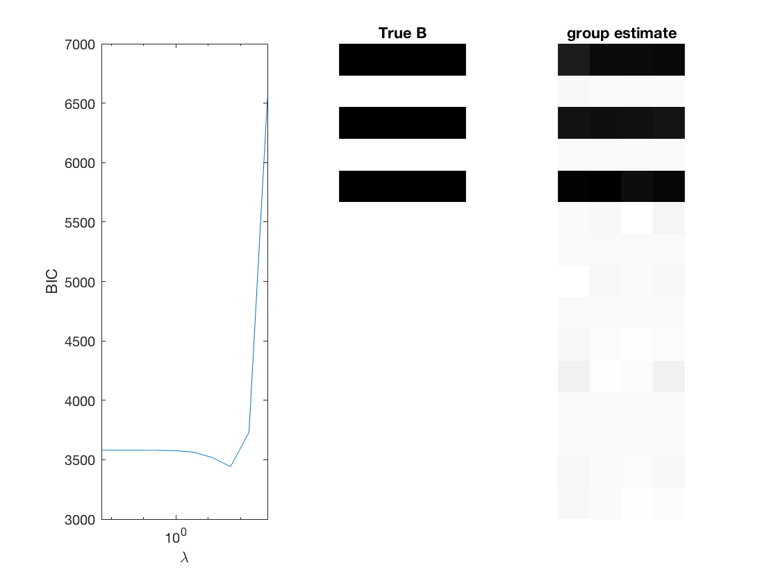
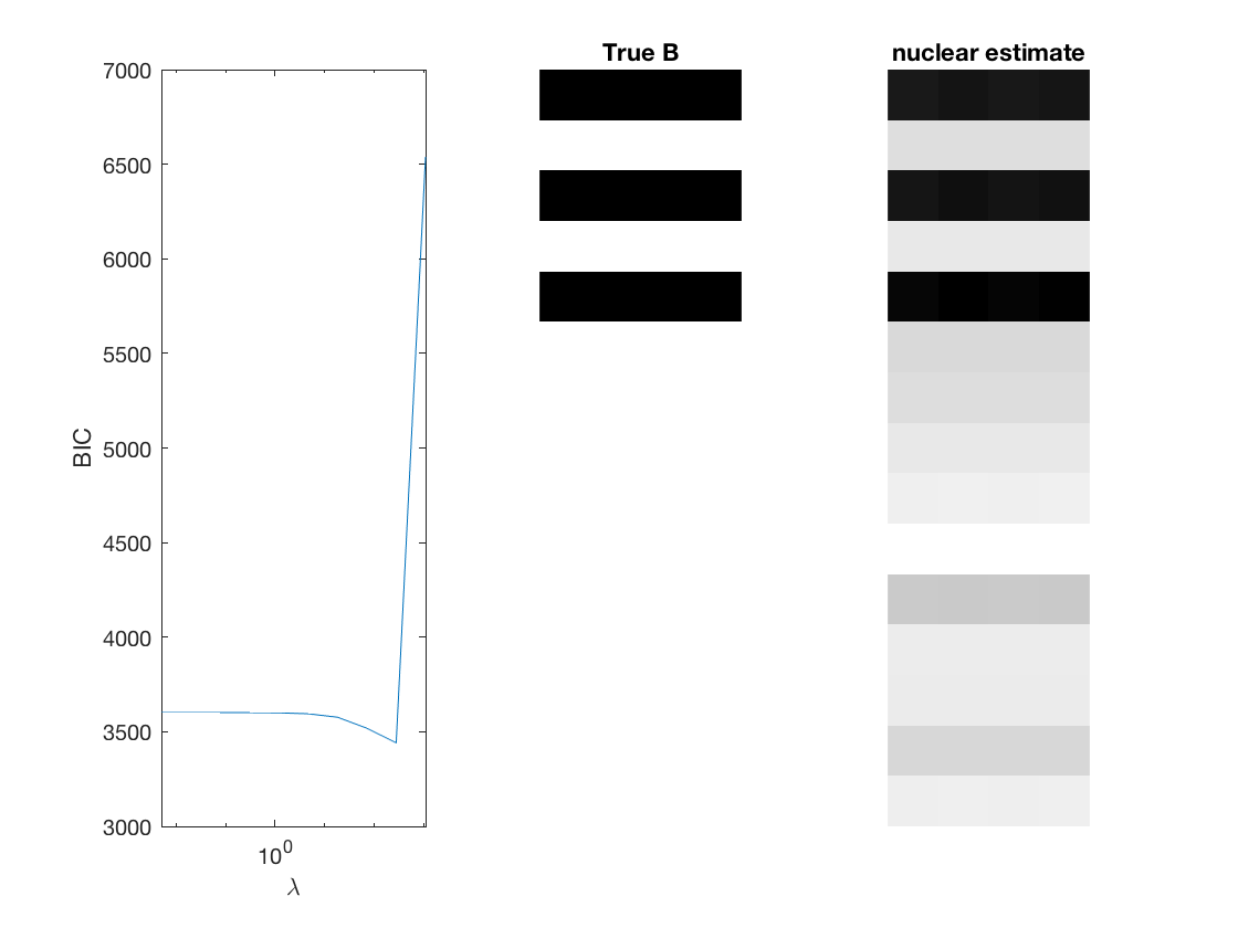
% True signal versus estimated signal
[bestbic,bestidx] = min(BICs);
B_best = mglm_sparsereg(X,Y,lambdas(bestidx),'penalty',pen,'dist',dist);
% display MSE of regularized estiamte
display(norm(B_best-B,2)/sqrt(numel(B)));
figure;
subplot(1,3,1);
semilogx(lambdas,BICs);
ylabel('BIC');
xlabel('\lambda');
xlim([min(lambdas) max(lambdas)]);
subplot(1,3,2);
imshow(mat2gray(-B)); title('True B');
subplot(1,3,3);
imshow(mat2gray(-B_best)); title([pen ' estimate']);
end
Elapsed time is 0.158750 seconds.
    0.0751

Elapsed time is 0.091532 seconds.
    0.0638

Elapsed time is 0.231174 seconds.
    0.1726