Negative multinomial regression and sparse regression
A demo of negative multinomial regression and sparse regression
Contents
- Generate negative multinomial random vectors from covariates
- Fit negative multinomial regression - link over-disperson parameter
- Fit negative multinomial regression - not linking over-disperson parameter
- Fit negative multinomial sparse regression - lasso/group/nuclear penalty
- Sparse regression (not linking over-disp.) - lasso/group/nuclear penalty
Generate negative multinomial random vectors from covariates
clear;
% reset random seed
s = RandStream('mt19937ar','Seed',1);
RandStream.setGlobalStream(s);
% sample size
n = 200;
% # covariates
p = 15;
% # bins
d = 5;
% design matrix
X = randn(n,p);
% true regression coefficients
B = zeros(p,d+1);
nzidx = [1 3 5];
B(nzidx,:) = ones(length(nzidx),d+1);
eta = X*B;
alpha = exp(eta);
prob(:,d+1) = 1./(sum(alpha(:,1:d),2)+1);
prob(:,1:d) = bsxfun(@times, alpha(:,1:d), prob(:,d+1));
b= binornd(10,0.2, n, 1);
Y = negmnrnd(prob,b);

zerorows = sum(Y,2);
Y=Y(zerorows~=0, :);
X=X(zerorows~=0, :);
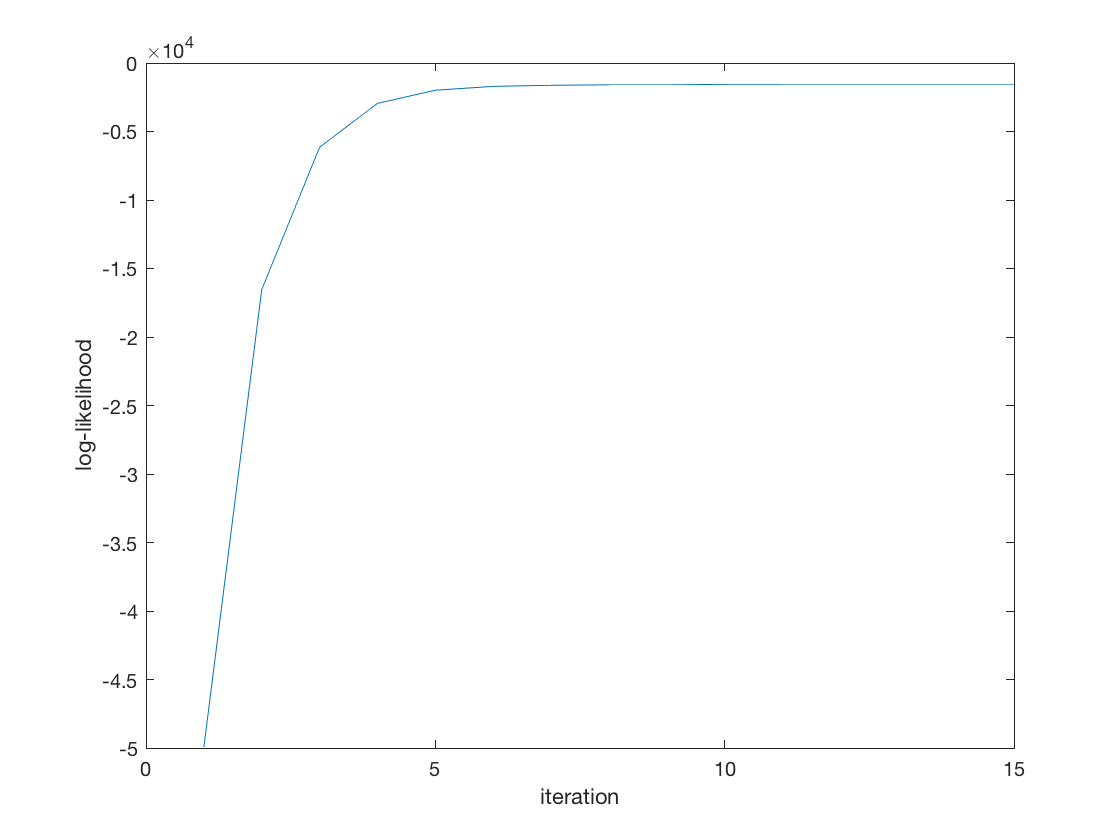
Fit negative multinomial regression - link over-disperson parameter
tic;
[B_hat, stats] = negmnreg(X,Y);
toc;
display(B_hat);
display(stats);
% Wald test of predictor significance
display('Wald test p-values:');
display(stats.wald_pvalue);

figure;
plot(stats.logL_iter);
xlabel('iteration');
ylabel('log-likelihood');
Elapsed time is 0.225574 seconds.

B_hat =

    1.0559    1.0459    1.0098    1.0084    0.9932   -0.1119
    0.0278   -0.0052    0.0070    0.0158    0.0092    0.1827
    0.8343    0.8947    0.9116    0.8642    0.8333    0.2859
    0.0411   -0.0185    0.0076   -0.0617   -0.0201    0.0264
    0.9650    1.0042    1.0083    1.0122    1.0710   -0.1664
   -0.1669   -0.1084   -0.0812   -0.1458   -0.0916    0.0577
   -0.1095   -0.0959   -0.0644   -0.1221   -0.0612    0.3709
    0.1659    0.1893    0.1286    0.1494    0.0899   -0.2356
   -0.0414    0.0081   -0.1278   -0.0591   -0.0835    0.2748
   -0.0397   -0.1438   -0.0578   -0.0818   -0.1170   -0.0070
    0.2200    0.3404    0.2959    0.2698    0.2547   -0.5784
    0.1163    0.1595    0.1778    0.0901    0.1181   -0.1753
   -0.1064   -0.0661   -0.1113   -0.0682   -0.0980    0.0240
    0.0613    0.0525    0.0720    0.0194    0.0251   -0.0206
   -0.0697   -0.0377    0.0490    0.0055   -0.0188    0.1182


stats =

  struct with fields:

                     BIC: 3.5447e+03
                     dof: 90
              iterations: 15
                    logL: -1.5451e+03
               logL_iter: [1×15 double]
                      se: [15×6 double]
               wald_stat: [1×15 double]
             wald_pvalue: [1×15 double]
                       H: [90×90 double]
                gradient: [90×1 double]
    observed_information: [90×90 double]

Wald test p-values:
  Columns 1 through 7

         0    0.6526         0    0.6493         0    0.4724    0.0606

  Columns 8 through 14

    0.2285    0.0125    0.4257    0.0038    0.4790    0.8500    0.9286

  Column 15

    0.3161
Fit negative multinomial regression - not linking over-disperson parameter
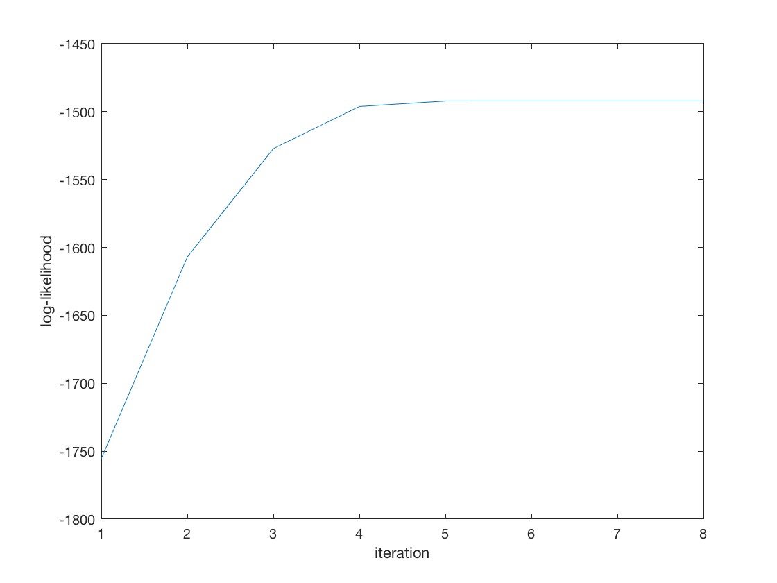
tic;
[B_hat, b_hat, stats] = negmnreg2(X,Y);
toc;
disp(B_hat);
disp(stats.se_B);
disp(b_hat);
disp(stats.se_b);
display(stats);
% Wald test of predictor significance
display('Wald test p-values:');
display(stats.wald_pvalue);

figure;
plot(stats.logL_iter);
xlabel('iteration');
ylabel('log-likelihood');
Elapsed time is 0.137911 seconds.
    0.8703    0.8610    0.8284    0.8264    0.8117
    0.1526    0.1215    0.1320    0.1414    0.1345
    0.9052    0.9645    0.9824    0.9348    0.9053
    0.0244   -0.0311   -0.0085   -0.0746   -0.0338
    0.7500    0.7874    0.7897    0.7939    0.8518
   -0.1307   -0.0742   -0.0470   -0.1106   -0.0575
    0.0262    0.0408    0.0669    0.0126    0.0717
    0.0421    0.0648    0.0063    0.0266   -0.0318
    0.0491    0.0947   -0.0345    0.0310    0.0079
   -0.0425   -0.1418   -0.0618   -0.0832   -0.1186
   -0.0724    0.0411    0.0022   -0.0252   -0.0394
    0.0828    0.1263    0.1437    0.0583    0.0849
   -0.1464   -0.1080   -0.1518   -0.1103   -0.1390
    0.0242    0.0186    0.0351   -0.0156   -0.0100
   -0.0008    0.0313    0.1110    0.0707    0.0458

    0.0760    0.0756    0.0756    0.0758    0.0758
    0.0757    0.0754    0.0755    0.0758    0.0757
    0.0672    0.0667    0.0666    0.0671    0.0671
    0.0768    0.0766    0.0765    0.0767    0.0766
    0.0765    0.0764    0.0763    0.0766    0.0763
    0.0660    0.0655    0.0660    0.0662    0.0660
    0.0699    0.0694    0.0694    0.0698    0.0697
    0.0617    0.0612    0.0614    0.0618    0.0614
    0.0712    0.0708    0.0709    0.0712    0.0709
    0.0745    0.0739    0.0738    0.0744    0.0742
    0.0752    0.0753    0.0750    0.0754    0.0755
    0.0679    0.0674    0.0673    0.0673    0.0674
    0.0722    0.0718    0.0720    0.0722    0.0722
    0.0671    0.0666    0.0670    0.0670    0.0670
    0.0692    0.0690    0.0687    0.0691    0.0688

    2.2915

    0.1355


stats =

  struct with fields:

                     BIC: 3.3630e+03
              iterations: 8
                    logL: -1.4921e+03
               logL_iter: [1×8 double]
                      se: [15×6 double]
               wald_stat: [1×15 double]
             wald_pvalue: [1×15 double]
                       H: [76×76 double]
                gradient: [76×1 double]
    observed_information: [76×76 double]
                    se_B: [15×5 double]
                    se_b: 0.1355

Wald test p-values:
  Columns 1 through 7

         0    0.4959         0    0.5382         0    0.3026    0.7689

  Columns 8 through 14

    0.2618    0.1964    0.2896    0.4888    0.1913    0.3636    0.8945

  Column 15

    0.3568
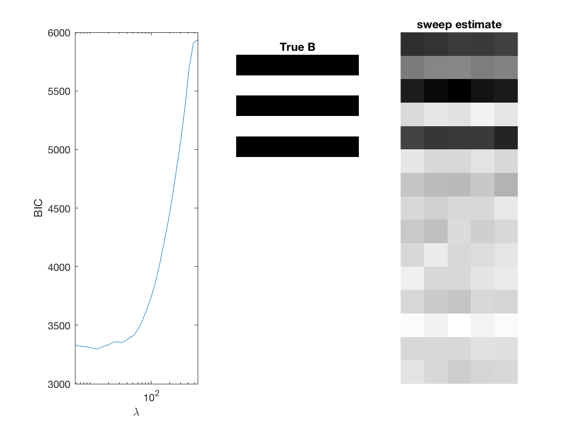
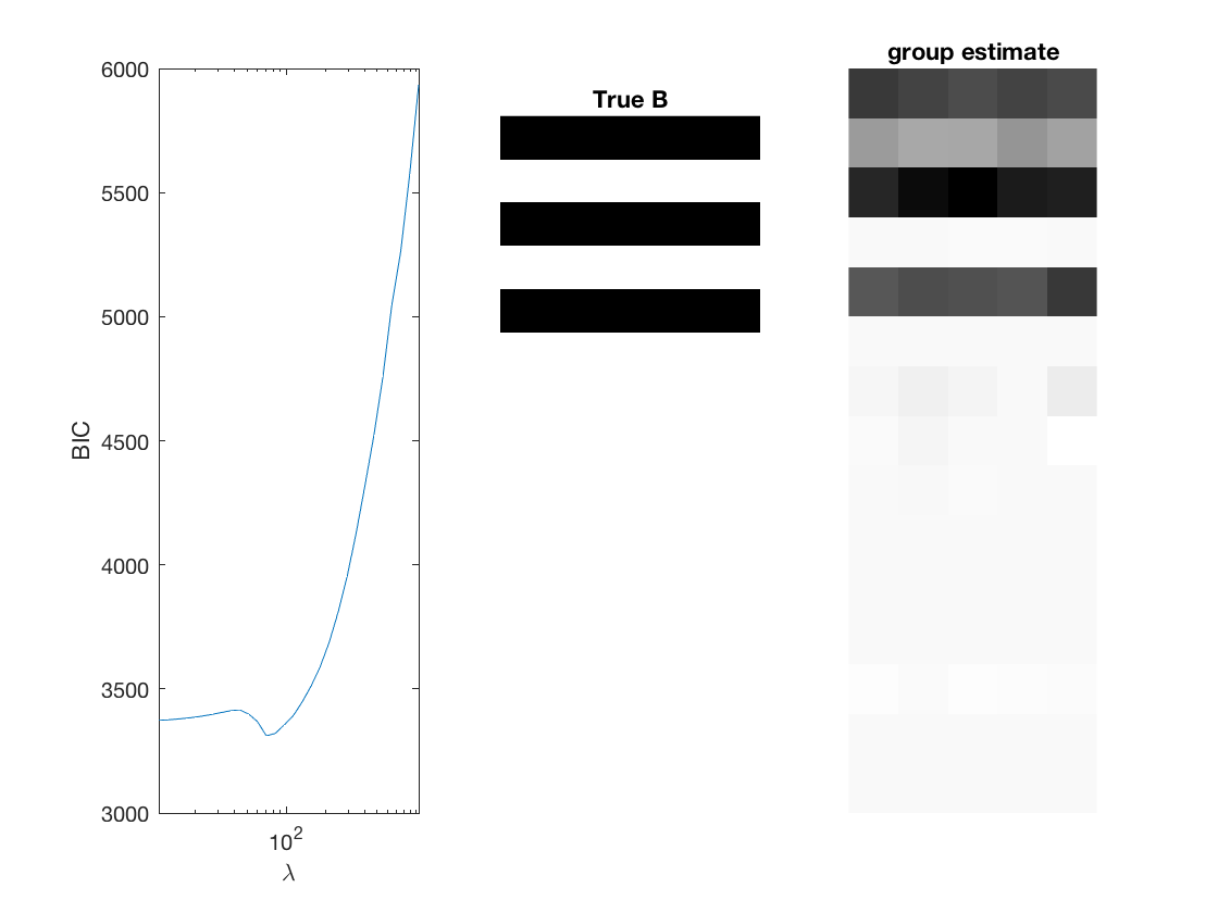
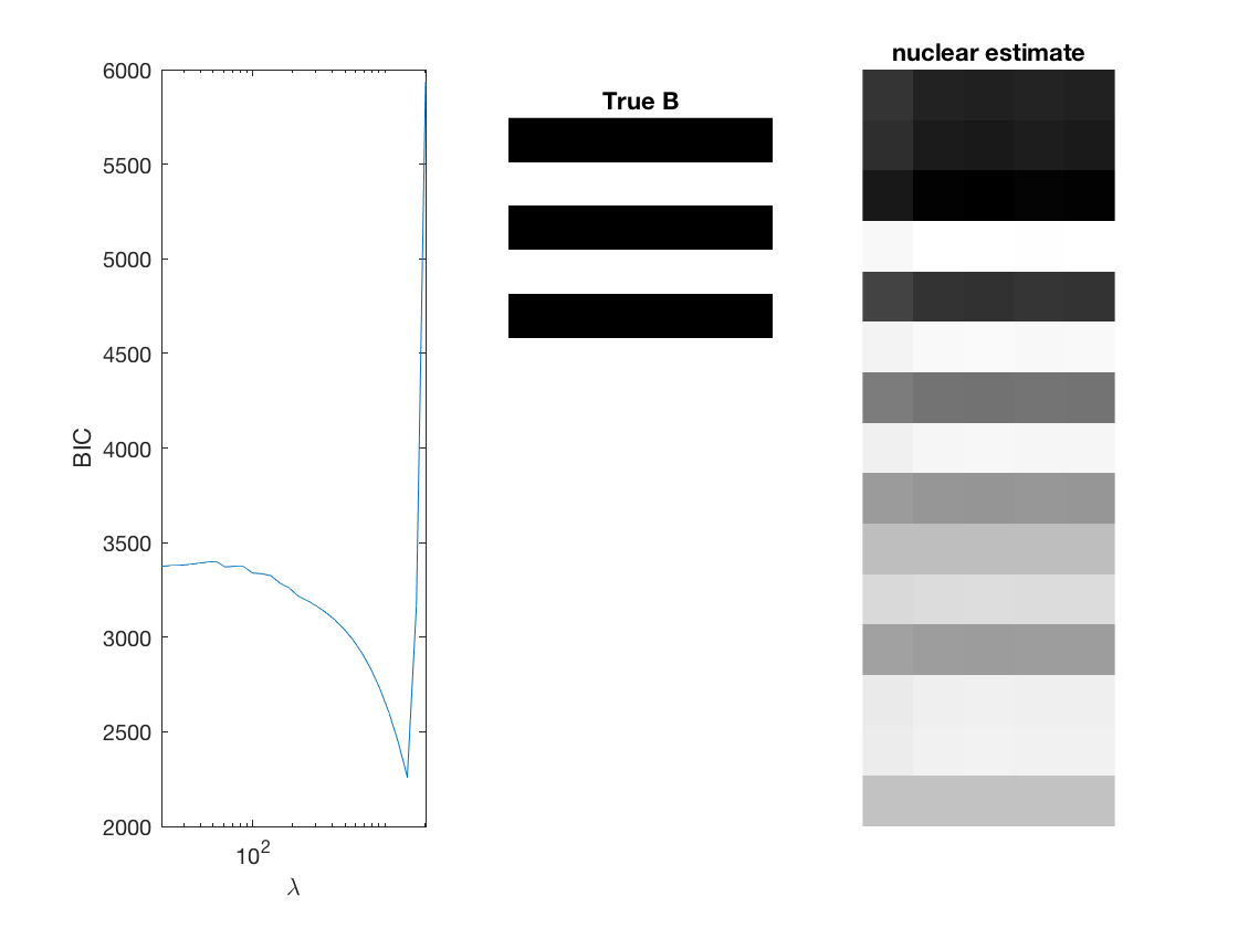
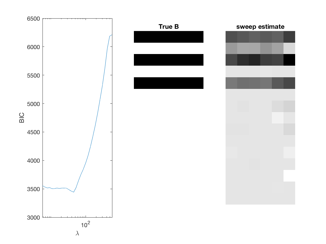
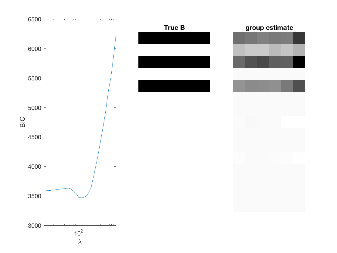
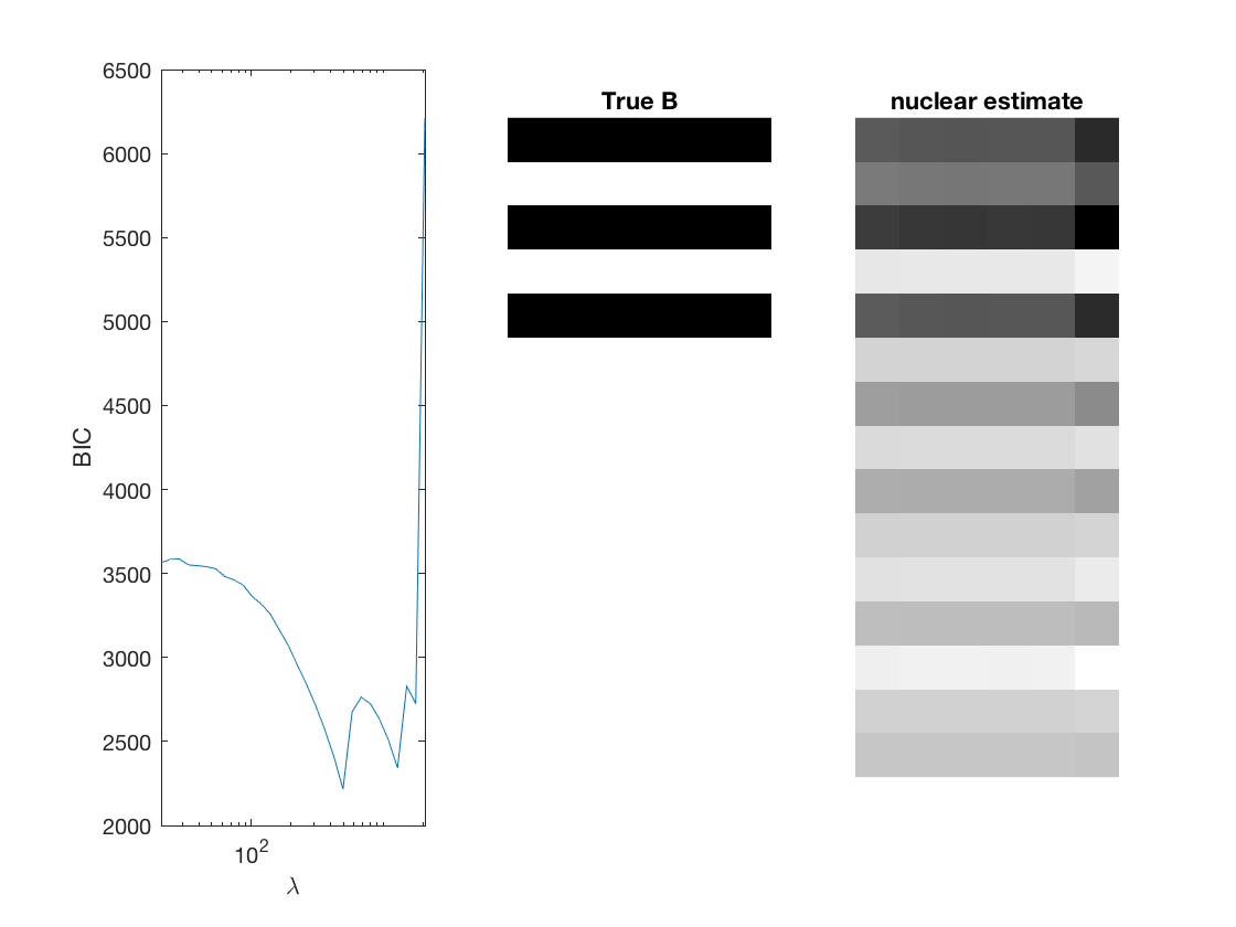
Fit negative multinomial sparse regression - lasso/group/nuclear penalty
Regression on the over dispersion parameter
penalty = {'sweep','group','nuclear'};
ngridpt = 30;
dist = 'negmn';

for i = 1:length(penalty)

    pen = penalty{i};
    [~, stats] = mglm_sparsereg(X,Y,inf,'penalty',pen,'dist',dist);
    maxlambda = stats.maxlambda;

    lambdas = exp(linspace(log(maxlambda),log(maxlambda/100),ngridpt));
    BICs = zeros(1,ngridpt);
    logl =zeros(1, ngridpt);
    dofs = zeros(1, ngridpt);
    tic;
    for j=1:ngridpt
        if j==1
            B0 = zeros(p,d+1);
        else
            B0 = B_hat;
        end
        [B_hat, stats] = mglm_sparsereg(X,Y,lambdas(j),'penalty',pen, ...
            'dist',dist,'B0',B0);
        BICs(j) = stats.BIC;
        logl(j) = stats.logL;
        dofs(j) = stats.dof;
    end
    toc;

    % True signal versus estimated signal
    [bestbic,bestidx] = min(BICs);
    [B_best,stats] = mglm_sparsereg(X,Y,lambdas(bestidx),'penalty',pen,'dist',dist);
    figure;
    subplot(1,3,1);
    semilogx(lambdas,BICs);
    ylabel('BIC');
    xlabel('\lambda');
    xlim([min(lambdas) max(lambdas)]);
    subplot(1,3,2);
    imshow(mat2gray(-B)); title('True B');
    subplot(1,3,3);
    imshow(mat2gray(-B_best)); title([pen ' estimate']);

end
Elapsed time is 1.808871 seconds.
Elapsed time is 1.867126 seconds.
Elapsed time is 2.656329 seconds.
Sparse regression (not linking over-disp.) - lasso/group/nuclear penalty
Do not run regression on the over dispersion parameter
penalty = {'sweep','group','nuclear'};
ngridpt = 30;
dist = 'negmn2';

for i = 1:length(penalty)

    pen = penalty{i};
    [~, stats] = mglm_sparsereg(X,Y,inf,'penalty',pen,'dist',dist);
    maxlambda = stats.maxlambda;

    lambdas = exp(linspace(log(maxlambda),log(maxlambda/100),ngridpt));
    BICs = zeros(1,ngridpt);
    logl =zeros(1, ngridpt);
    dofs = zeros(1, ngridpt);
    tic;
    for j=1:ngridpt
        if j==1
            B0 = zeros(p,d);
        else
            B0 = B_hat;
        end
        [B_hat, stats] = mglm_sparsereg(X,Y,lambdas(j),'penalty',pen, ...
            'dist',dist,'B0',B0);
        BICs(j) = stats.BIC;
        logl(j) = stats.logL;
        dofs(j) = stats.dof;
    end
    toc;

    % True signal versus estimated signal
    [bestbic,bestidx] = min(BICs);
    B_best = mglm_sparsereg(X,Y,lambdas(bestidx),'penalty',pen,'dist',dist);
    figure;
    subplot(1,3,1);
    semilogx(lambdas,BICs);
    ylabel('BIC');
    xlabel('\lambda');
    xlim([min(lambdas) max(lambdas)]);
    subplot(1,3,2);
    imshow(mat2gray(-B)); title('True B');
    subplot(1,3,3);
    imshow(mat2gray(-B_best)); title([pen ' estimate']);

end
Elapsed time is 4.949842 seconds.
Elapsed time is 4.714719 seconds.
Elapsed time is 5.183260 seconds.