Contents

Regularized matrix linear regression

clear;
% reset random seed
s = RandStream('mt19937ar','Seed',2);
RandStream.setGlobalStream(s);

True coefficients for regular (non-array) covariates

p0 = 5;
b0 = ones(p0,1);

2D true signal: 64-by-64 cross

shape = imread('cross.gif');
shape = array_resize(shape,[32,32]); % 32-by-32
b = zeros(2*size(shape));
b((size(b,1)/4):(size(b,1)/4)+size(shape,1)-1, ...
    (size(b,2)/4):(size(b,2)/4)+size(shape,2)-1) = shape;
[p1,p2] = size(b);
disp(size(b));

    64    64

Simulate covariates

n = 500;    % sample size
X = randn(n,p0);   % n-by-p0 regular design matrix
M = tensor(randn(p1,p2,n));  % p1-by-p2-by-n matrix variates
disp(size(M));

    64    64   500

Simulate responses

mu = X*b0 + double(ttt(tensor(b), M, 1:2));
sigma = 1;  % noise level
y = mu + sigma*randn(n,1);

Determine max lambda to start

[~,~,stats] = matrix_sparsereg(X,M,y,inf,'normal');
maxlambda = stats.maxlambda*.95;

Fit nuclear norm regularized linear regression at grid points

gridpts = 10;
lambdas = zeros(1,gridpts);
gs = 2/(1+sqrt(5));
B = cell(1,gridpts);
AIC = zeros(1,gridpts);
BIC = zeros(1,gridpts);
tic;
for i=1:gridpts
    if (i==1)
        B0 = [];
    else
        B0 = B{i-1};    % warm start
    end
    lambda = maxlambda*gs^(i-1);
    lambdas(i) = lambda;
    [beta0,B{i},stats] = matrix_sparsereg(X,M,y,lambda,'normal','B0',B0);
    AIC(i) = stats.AIC;
    BIC(i) = stats.BIC;
end
toc;

Elapsed time is 0.935886 seconds.

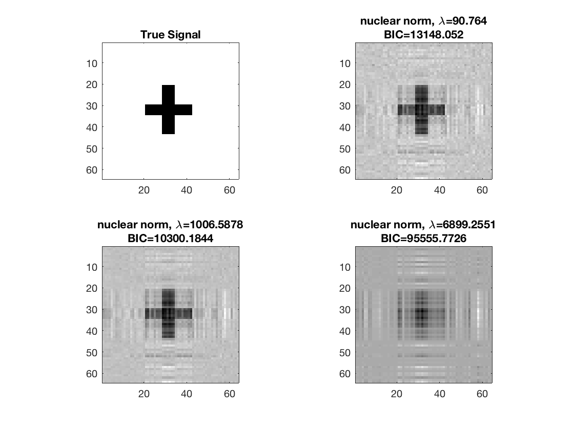
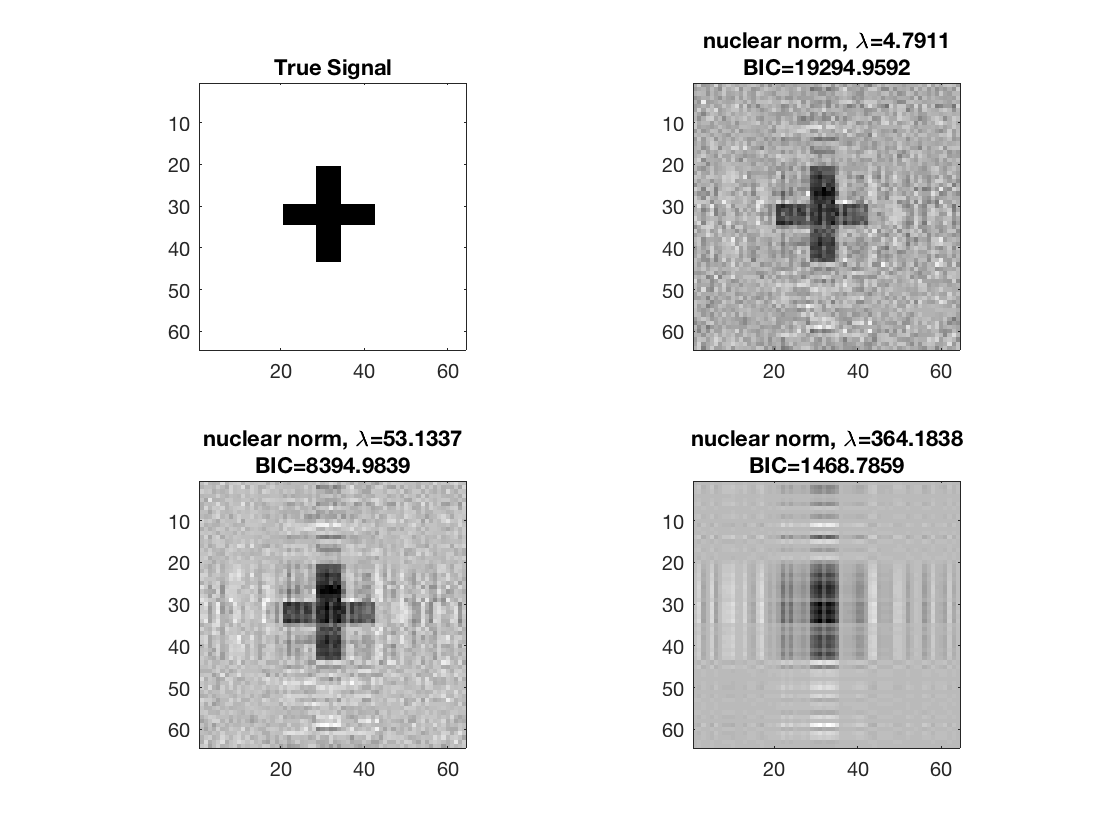
disp true signal and snapshots along nuclear norm solution path

figure; hold on;
set(gca,'FontSize',20);

subplot(2,2,1);
imagesc(-b);
colormap(gray);
title('True Signal');
axis equal;
axis tight;

ploti = 1;
for i=[gridpts round(gridpts/2) 1]
    ploti = ploti + 1;
    subplot(2,2,ploti);
    imagesc(-double(B{i}));
    colormap(gray);
    title({['nuclear norm,', ' \lambda=', ...
        num2str(lambdas(i))]; ['BIC=', num2str(BIC(i))]});
    axis equal;
    axis tight;
end

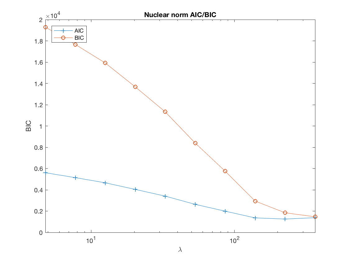
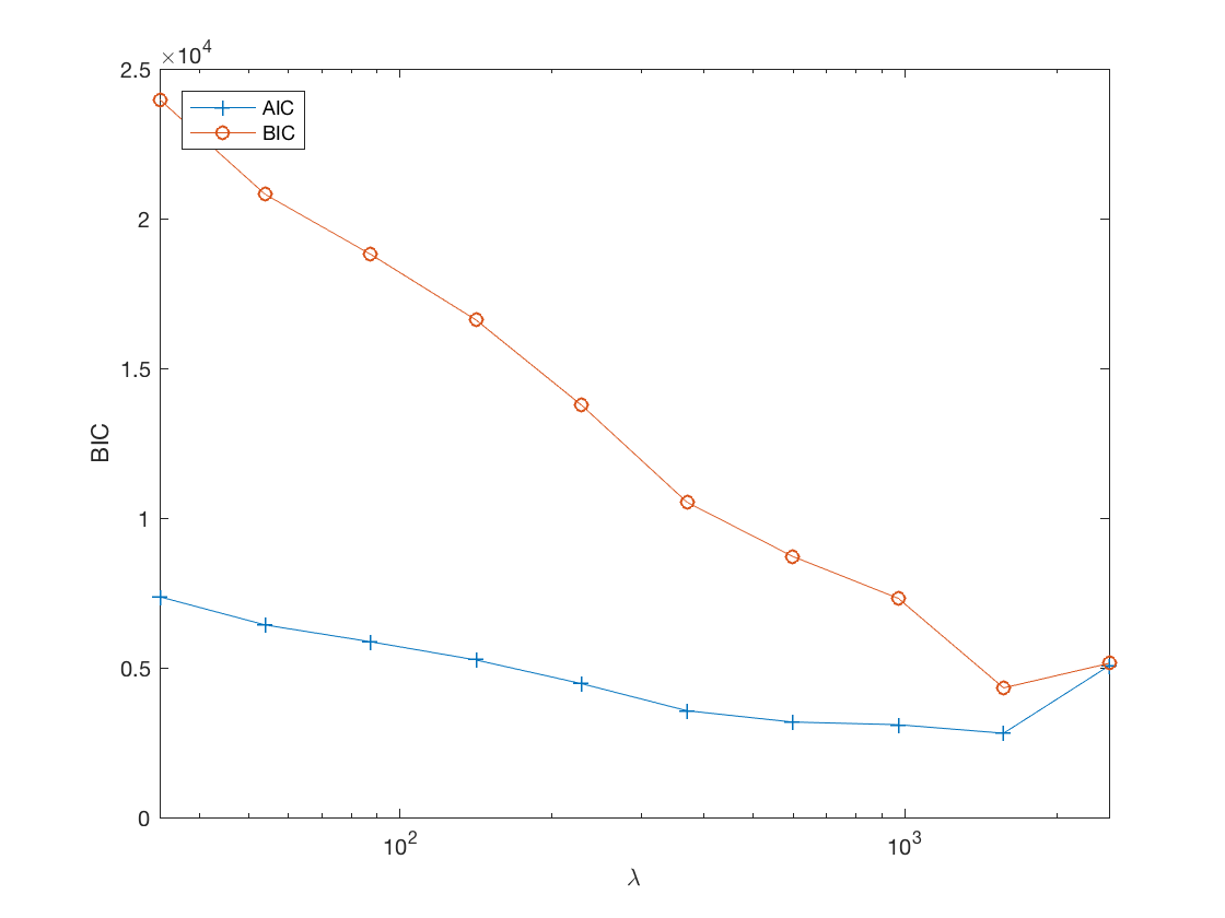
disp AIC/BIC trace plot

figure;
set(gca,'FontSize',20);
semilogx(lambdas, AIC, '-+', lambdas, BIC, '-o');
xlabel('\lambda');
ylabel('BIC');
xlim([min(lambdas) max(lambdas)]);
title('Nuclear norm AIC/BIC');
legend('AIC', 'BIC', 'Location', 'northwest');

Compare to lasso penalized linear regression

Transform matrix variates to vector form

TM = tenmat(tensor(M),3,[1 2]);
Xall = [double(TM) X];

Determine max lambda to start

lambdastart = max(lsq_maxlambda(sum(Xall.^2),-y'*Xall,'enet',1));
maxlambda_lasso = lambdastart*.95;

Optimization at grid points

gridpts = 10;
B_lasso = cell(1,gridpts);
BIC_lasso = zeros(1,gridpts);
lambdas_lasso = zeros(1,gridpts);
penidx = true(size(Xall,2),1);
penidx(numel(b)+1:end) = false; % do not penalize regular covariates

tic;
for i=1:gridpts
    if (i==1)
        x0 = zeros(size(Xall,2),1);
    else
        x0 = beta;
    end
    lambda = maxlambda_lasso*gs^(i-1);
    lambdas_lasso(i) = lambda;
    [beta] = lsq_sparsereg(Xall,y,lambda,'x0',x0,'penidx',penidx);
    B_lasso{i} = reshape(beta(1:numel(b)),p1,p2);
    BIC_lasso(i) = .5*norm(y-Xall*beta)^2+log(n)*nnz(abs(beta)>1e-8);
end
toc;

Elapsed time is 4.505069 seconds.

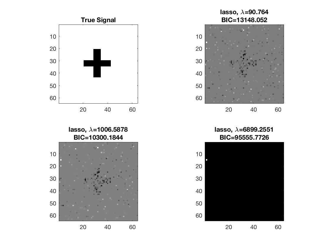
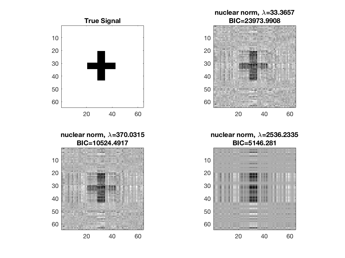
disp true signal and snapshots along lasso solution path

figure; hold on;
set(gca,'FontSize',20);

subplot(2,2,1);
imagesc(-b);
colormap(gray);
title('True Signal');
axis equal;
axis tight;

ploti = 1;
for i=[gridpts round(gridpts/2) 1]
    ploti = ploti + 1;
    subplot(2,2,ploti);
    imagesc(-B_lasso{i});
    colormap(gray);
    title({['lasso' ', \lambda=', ...
        num2str(lambdas(i))]; ['BIC=', num2str(BIC(i))]});
    axis equal;
    axis tight;
end

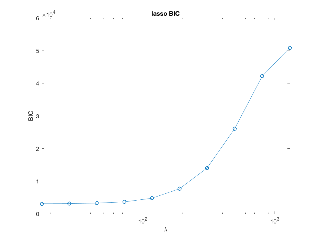
Lasso BIC path

figure;
set(gca,'FontSize',20);
semilogx(lambdas_lasso,BIC_lasso,'-o');
title('lasso BIC');
xlabel('\lambda');
ylabel('BIC');
xlim([min(lambdas_lasso),max(lambdas_lasso)]);

Regularized matrix Poisson (log-linear) regression

clear;
% reset random seed
s = RandStream('mt19937ar','Seed',2);
RandStream.setGlobalStream(s);

2D true signal: 64-by-64 cross

shape = imread('cross.gif');
shape = array_resize(shape,[32,32]); % 32-by-32
b = zeros(2*size(shape));
b((size(b,1)/4):(size(b,1)/4)+size(shape,1)-1, ...
    (size(b,2)/4):(size(b,2)/4)+size(shape,2)-1) = shape;
[p1,p2] = size(b);
disp(size(b));

    64    64

True coefficients for regular (non-array) covariates

p0 = 5;
b0 = ones(p0,1);

Simulate covariates

n = 750;    % sample size
X = randn(n,p0);   % n-by-p regular design matrix
M = tensor(randn(p1,p2,n));  % n p1-by-p2 matrix variates
disp(size(M));

% Simulate Poisson count responses from the systematic components
mu = X*b0 + double(ttt(tensor(b), M, 1:2));
mu = mu/(max(abs(mu)))*5;   % scale to [-5, 5], to avoid overflow
y = poissrnd(exp(mu));

    64    64   750

Determine max lambda to start

[~,~,stats] = matrix_sparsereg(X,M,y,inf,'poisson');
maxlambda = stats.maxlambda*.95;

Fit nuclear norm regularized Poisson regression at grid points

gridpts = 10;
lambdas = zeros(1,gridpts);
gs = 2/(1+sqrt(5));
B = cell(1,gridpts);
AIC = zeros(1,gridpts);
BIC = zeros(1,gridpts);
tic;
for i=1:gridpts
    if (i==1)
        B0 = [];
    else
        B0 = B{i-1};
    end
    lambda = maxlambda*gs^(i-1);
    lambdas(i) = lambda;
    [beta0,B{i},stats] = matrix_sparsereg(X,M,y,lambda,'poisson','B0',B0);
    AIC(i) = stats.AIC;
    BIC(i) = stats.BIC;
end
toc

Elapsed time is 2.569610 seconds.

disp true signal and snapshots along nuclear norm solution path

figure; hold on;
set(gca,'FontSize',20);

subplot(2,2,1);
imagesc(-b);
colormap(gray);
title('True Signal');
axis equal;
axis tight;

ploti = 1;
for i=[gridpts round(gridpts/2) 1]
    ploti = ploti + 1;
    subplot(2,2,ploti);
    imagesc(-double(B{i}));
    colormap(gray);
    title({['nuclear norm,', ' \lambda=', ...
        num2str(lambdas(i))]; ['BIC=', num2str(BIC(i))]});
    axis equal;
    axis tight;
end

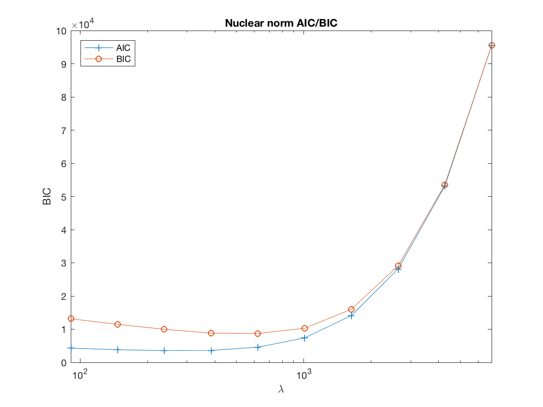
disp AIC/BIC trace plot

figure;
set(gca,'FontSize',20);
semilogx(lambdas, AIC, '-+', lambdas, BIC, '-o');
xlabel('\lambda');
ylabel('BIC');
xlim([min(lambdas) max(lambdas)]);
legend('AIC', 'BIC', 'Location', 'northwest');

% %% Compare to lasso penalized Poisson (log-linear) regression
%
% %%
% % Transform matrix variates to vector form
% TM = tenmat(tensor(M),3,[1 2]);
% Xall = [double(TM) X];
%
% %%
% % Determine max lambda to start
% lambdastart = 0;
% for j=1:numel(b)
%     lambdastart = max(lambdastart,glm_maxlambda(Xall(:,j),y,'loglinear'));
% end
% maxlambda_lasso = lambdastart*.95;
%
% %%
% % Optimization at grid points
% gridpts = 10;
% B_lasso = cell(1,gridpts);
% BIC_lasso = zeros(1,gridpts);
% lambdas_lasso = zeros(1,gridpts);
% penidx = true(size(Xall,2),1);
% penidx(numel(b)+1:end) = false; % do not penalize regular covariates
%
% tic;
% for i=1:gridpts
%     if (i==1)
%         x0 = zeros(size(Xall,2),1);
%     else
%         x0 = beta;
%     end
%     lambda = maxlambda_lasso*gs^(i-1);
%     lambdas_lasso(i) = lambda;
%     [beta] = glm_sparsereg(Xall,y,lambda,'loglinear', ...
%         'x0',x0,'penidx',penidx);
%     B_lasso{i} = beta(1:numel(b));
%     eta = Xall*beta;
%     BIC_lasso(i) = - sum(y.*log(eta)-gammaln(y+1)-eta) ...
%         + log(n)*nnz(abs(beta)>1e-8);
% end
% toc;
%
% %%
% % disp true sinal and snapshots along lasso solution path
% figure; hold on;
% set(gca,'FontSize',20);
%
% subplot(2,2,1);
% imagesc(-b);
% colormap(gray);
% title('True Signal');
% axis equal;
% axis tight;
%
% ploti = 1;
% for i=[gridpts round(gridpts/2) 1]
%     ploti = ploti + 1;
%     subplot(2,2,ploti);
%     imagesc(-reshape(B_lasso{i},p1,p2));
%     colormap(gray);
%     title({['lasso' ', \lambda=', ...
%         num2str(lambdas(i))]; ['BIC=', num2str(BIC(i))]});
%     axis equal;
%     axis tight;
% end
%
% %%
% % Lasso BIC path
% figure;
% set(gca,'FontSize',20);
% semilogx(lambdas_lasso,BIC_lasso,'-o');
% title('lasso BIC');
% xlabel('\lambda');
% ylabel('BIC');
% xlim([min(lambdas_lasso),max(lambdas_lasso)]);

Regularized matrix logistic regression

clear;
% reset random seed
s = RandStream('mt19937ar','Seed',2);
RandStream.setGlobalStream(s);

2D true signal: 64-by-64 cross

shape = imread('cross.gif');
shape = array_resize(shape,[32,32]); % 32-by-32
b = zeros(2*size(shape));
b((size(b,1)/4):(size(b,1)/4)+size(shape,1)-1, ...
    (size(b,2)/4):(size(b,2)/4)+size(shape,2)-1) = shape;
[p1,p2] = size(b);
disp(size(b));

    64    64

True coefficients for regular (non-array) covariates

p0 = 5;
b0 = ones(p0,1);

Simulate covariates

n = 1000;    % sample size
X = randn(n,p0);   % n-by-p regular design matrix
M = tensor(randn(p1,p2,n));  % n p1-by-p2 matrix variates
disp(size(M));

          64          64        1000

Simulate binary responses from the systematic components

mu = X*b0 + double(ttt(tensor(b), M, 1:2));
y = binornd(1, 1./(1+exp(-mu)));

Determine max lambda to start

[~,~,stats] = matrix_sparsereg(X,M,y,inf,'binomial');
maxlambda = stats.maxlambda*0.95;

Fit nuclear norm regularized logistic regression at grid points

gridpts = 10;
lambdas = zeros(1,gridpts);
gs = 2/(1+sqrt(5));
B = cell(1,gridpts);
AIC = zeros(1,gridpts);
BIC = zeros(1,gridpts);

tic;
for i=1:gridpts
    if (i==1)
        B0 = [];
    else
        B0 = B{i-1};
    end
    lambda = maxlambda*gs^(i-1);
    lambdas(i) = lambda;
    [beta0,B{i},stats] = matrix_sparsereg(X,M,y,lambda,'binomial','B0',B0);
    AIC(i) = stats.AIC;
    BIC(i) = stats.BIC;
end
toc

Elapsed time is 1.822904 seconds.

disp true signal and and snapshots along nuclear norm solution path

figure; hold on;
set(gca,'FontSize',20);

subplot(2,2,1);
imagesc(-b);
colormap(gray);
title('True Signal');
axis equal;
axis tight;

ploti = 1;
for i=[gridpts round(gridpts/2) 1]
    ploti = ploti + 1;
    subplot(2,2,ploti);
    imagesc(-double(B{i}));
    colormap(gray);
    title({['nuclear norm,', ' \lambda=', ...
        num2str(lambdas(i))]; ['BIC=', num2str(BIC(i))]});
    axis equal;
    axis tight;
end

disp AIC/BIC trace plot

figure;
set(gca,'FontSize',20);
semilogx(lambdas, AIC, '-+', lambdas, BIC, '-o');
xlabel('\lambda');
ylabel('BIC');
xlim([min(lambdas) max(lambdas)]);
title('Nuclear norm AIC/BIC');
legend('AIC', 'BIC', 'Location', 'northwest');

% %% Compare to lasso penalized logistic regression
%
% %%
% % Transform matrix variates to vector form
% TM = tenmat(tensor(M),3,[1 2]);
% Xall = [double(TM) X];
%
% %%
% % Determine max lambda to start
% lambdastart = 0;            % find the maximum tuning parameter to start
% for j=1:numel(b)
%     lambdastart = max(lambdastart,glm_maxlambda(Xall(:,j),y,'logistic'));
% end
% maxlambda_lasso = lambdastart;
%
% %%
% % Optimization at grid points
% gridpts = 10;
% B_lasso = cell(1,gridpts);
% BIC_lasso = zeros(1,gridpts);
% lambdas_lasso = zeros(1,gridpts);
% penidx = true(size(Xall,2),1);
% penidx(numel(b)+1:end) = false; % do not penalize regular covariates
%
% tic;
% for i=1:gridpts
%     if (i==1)
%         x0 = zeros(size(Xall,2),1);
%     else
%         x0 = beta;
%     end
%     lambda = maxlambda_lasso*gs^(i-1);
%     lambdas_lasso(i) = lambda;
%     [beta] = glm_sparsereg(Xall,y,lambda,'logistic','x0',x0, ...
%         'penidx',penidx);
%     B_lasso{i} = beta(1:numel(b));
%     eta = Xall*beta;
%     BIC_lasso(i) = - sum(y.*eta-log(1+exp(eta))) ...
%         + log(n)*nnz(abs(beta)>1e-8);
% end
% toc;
%
% %%
% % disp true signal and snapshots along lasso solution path
% figure; hold on;
% set(gca,'FontSize',20);
%
% subplot(2,2,1);
% imagesc(-b);
% colormap(gray);
% title('True Signal');
% axis equal;
% axis tight;
%
% ploti = 1;
% for i=[gridpts round(gridpts/2) 1]
%     ploti = ploti + 1;
%     subplot(2,2,ploti);
%     imagesc(-reshape(B_lasso{i},p1,p2));
%     colormap(gray);
%     title({['lasso' ', \lambda=', ...
%         num2str(lambdas(i))]; ['BIC=', num2str(BIC(i))]});
%     axis equal;
%     axis tight;
% end
%
% %%
% % Lasso BIC path
% figure;
% set(gca,'FontSize',20);
% semilogx(lambdas_lasso,BIC_lasso,'-o');
% title('lasso BIC');
% xlabel('\lambda');
% ylabel('BIC');
% xlim([min(lambdas_lasso),max(lambdas_lasso)]);

Published with MATLAB® R2017a