Quasi-Newton Method (KL 14.9)

Introduction

• Quasi-Newton is one of the most successful "black-box" optimizers in use.

  • Optim.jl, NLopt.jl, Ipopt.jl packages in Julia.
  • optim in R.

• Consider the general Newton scheme for minimizing $f(\mathbf{x})$, $\mathbf{x} \in {\cal \mathbf{X}} \subset \mathbb{R}^p$:
  $$ \mathbf{x}^{(t+1)} = \mathbf{x}^{(t)} - s [\mathbf{A}^{(t)}]^{-1} \nabla f(\mathbf{x}^{(t)}), $$ where $\mathbf{A}^{(t)}$ a pd approximation of the Hessian $d^2 f(\mathbf{x}^{(t)})$.

  • Pros: fast convergence
  • Cons: compute and store Hessian at each iteration (usually $O(np^2)$ cost in statistical problems), solving a linear system ($O(p^3)$ cost in general), human efforts (derive and implement gradient and Hessian, pd approximation, ...)

• Any pd $\mathbf{A}$ gives a descent algorithm - tradeoff between convergence rate and cost per iteration.

• Setting $\mathbf{A} = \mathbf{I}$ leads to the steepest descent algorithm. Picture: slow convergence (zig-zagging) of steepest descent (with exact line search) for minimizing a convex quadratic function (ellipse).

How many steps does the Newton's method using the Hessian take for a convex quadratic $f$?

Quasi-Newton

• Idea of Quasi-Newton: No analytical Hessian is required (still need gradient). Bootstrap Hessian from gradient!

• Update approximate Hessian $\mathbf{A}$ according to the secant condition $$ \begin{eqnarray*} \nabla f(\mathbf{x}^{(t)}) - \nabla f(\mathbf{x}^{(t-1)}) \approx [d^2 f(\mathbf{x}^{(t)})] (\mathbf{x}^{(t)} - \mathbf{x}^{(t-1)}). \end{eqnarray*} $$ Instead of computing $\mathbf{A}$ from scratch at each iteration, we update an approximation $\mathbf{A}$ to $d^2 f(\mathbf{x})$ that satisfies

  1. p.d.,
  2. the secant condition, and
  3. closest to the previous approximation.

• Super-linear convergence, compared to the quadratic convergence of Newton's method. But each iteration only takes $O(p^2)$!

• Davidon-Fletcher-Powell (DFP) rank-2 update. Solve $$ \begin{eqnarray*} &\text{minimize}& \, \|\mathbf{A} - \mathbf{A}^{(t)}\|_{\text{F}} \\ &\text{subject to}& \, \mathbf{A} = \mathbf{A}^T \\ & & \mathbf{A} (\mathbf{x}^{(t)}-\mathbf{x}^{(t-1)}) = \nabla f(\mathbf{x}^{(t)}) - \nabla f(\mathbf{x}^{(t-1)}) \end{eqnarray*} $$ for the next approximation $\mathbf{A}^{(t+1)}$. The solution is a low rank (rank 1 or rank 2) update of $\mathbf{A}^{(t)}$. The inverse is too thanks to the Sherman-Morrison-Woodbury formula! $O(p^2)$ operations. Need to store a $p$-by-$p$ dense matrix. Positive definiteness is guaranteed by the same trick you will be using in HW4! See KL 14.9 for details.

• Broyden-Fletcher-Goldfarb-Shanno (BFGS) rank 2 update is considered by many the most effective among all quasi-Newton updates. BFGS imposes secant condition on the inverse of Hessian $\mathbf{H} = \mathbf{A}^{-1}$. $$ \begin{eqnarray*} &\text{minimize}& \, \|\mathbf{H} - \mathbf{H}^{(t)}\|_{\text{F}} \\ &\text{subject to}& \, \mathbf{H} = \mathbf{H}^T \\ & & \mathbf{H} [ \nabla f(\mathbf{x}^{(t)}) - \nabla f(\mathbf{x}^{(t-1)})] = \mathbf{x}^{(t)}-\mathbf{x}^{(t-1)}. \end{eqnarray*} $$ Again $\mathbf{H}^{(t+1)}$ is a rank two update of $\mathbf{H}^{(t)}$. $O(p^2)$ operations. Still need to store a dense $p$-by-$p$ matrix.

• Limited-memory BFGS (L-BFGS). Only store the secant pairs. No need to store the $p$-by-$p$ approximate inverse Hessian. Particularly useful for large scale optimization.

• How to set the initial approximation $\mathbf{A}^{(0)}$? Identity or Hessian (if pd) or Fisher information matrix at starting point.

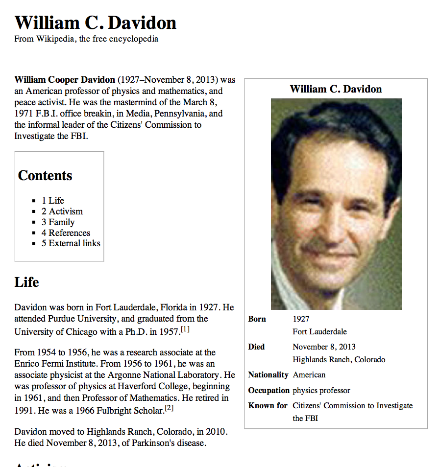
• History: Davidon was a physicist at Argonne National Lab in 1950s and proposed the very first idea of quasi-Newton method in 1959. Later studied, implemented, and popularized by Fletcher and Powell. Davidon's original paper was not accepted for publication 😞; 30 years later it appeared as the first article in the inaugural issue of SIAM Journal of Optimization.

Examples

Let's try different optimization algorithms on the handwritten digit example (HW4).