Optimization Examples - Semidefinite Programming (SDP)
SDP
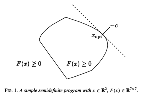
A semidefinite program (SDP) has the form \begin{eqnarray*} &\text{minimize}& \mathbf{c}^T \mathbf{x} \\ &\text{subject to}& x_1 \mathbf{F}_1 + \cdots + x_n \mathbf{F}_n + \mathbf{G} \preceq \mathbf{0} \quad (\text{LMI, linear matrix inequality}) \\ & & \mathbf{A} \mathbf{x} = \mathbf{b}, \end{eqnarray*} where $\mathbf{G}, \mathbf{F}_1, \ldots, \mathbf{F}_n \in \mathbf{S}^k$, $\mathbf{A} \in \mathbb{R}^{p \times n}$, and $\mathbf{b} \in \mathbb{R}^p$.
When $\mathbf{G}, \mathbf{F}_1, \ldots, \mathbf{F}_n$ are all diagonal, SDP reduces to LP.
The standard form SDP has form \begin{eqnarray*} &\text{minimize}& \text{tr}(\mathbf{C} \mathbf{X}) \\ &\text{subject to}& \text{tr}(\mathbf{A}_i \mathbf{X}) = b_i, \quad i = 1, \ldots, p \\ & & \mathbf{X} \succeq \mathbf{0}, \end{eqnarray*} where $\mathbf{C}, \mathbf{A}_1, \ldots, \mathbf{A}_p \in \mathbf{S}^n$.
An inequality form SDP has form \begin{eqnarray*} &\text{minimize}& \mathbf{c}^T \mathbf{x} \\ &\text{subject to}& x_1 \mathbf{A}_1 + \cdots + x_n \mathbf{A}_n \preceq \mathbf{B}, \end{eqnarray*} with variable $\mathbf{x} \in \mathbb{R}^n$, and parameters $\mathbf{B}, \mathbf{A}_1, \ldots, \mathbf{A}_n \in \mathbf{S}^n$, $\mathbf{c} \in \mathbb{R}^n$.
Exercise. Write LP, QP, QCQP, and SOCP in form of SDP.
SDP example: nearest correlation matrix
- Let $\mathbb{C}^n$ be the convex set of $n \times n$ correlation matrices
\begin{eqnarray*}
\mathbb{C}^n = \{ \mathbf{X} \in \mathbf{S}_+^n: x_{ii}=1, i=1,\ldots,n\}.
\end{eqnarray*}
Given $\mathbf{A} \in \mathbf{S}^n$, often we need to find the closest correlation matrix to $\mathbf{A}$
\begin{eqnarray*}
&\text{minimize}& \|\mathbf{A} - \mathbf{X}\|_{\text{F}} \\
&\text{subject to}& \mathbf{X} \in \mathbb{C}^n.
\end{eqnarray*}
This projection problem can be solved via an SDP
\begin{eqnarray*}
&\text{minimize}& t \\
&\text{subject to}& \|\mathbf{A} - \mathbf{X}\|_{\text{F}} \le t \\
& & \mathbf{X} = \mathbf{X}^T, \, \text{diag}(\mathbf{X}) = \mathbf{1} \\
& & \mathbf{X} \succeq \mathbf{0}
\end{eqnarray*}
in variables $\mathbf{X} \in \mathbb{R}^{n \times n}$ and $t \in \mathbb{R}$. The SOC constraint can be written as an LMI
\begin{eqnarray*}
\begin{pmatrix}
\end{pmatrix} \succeq \mathbf{0} \end{eqnarray*} by the Schur complement lemma.t \mathbf{I} & \text{vec} (\mathbf{A} - \mathbf{X}) \\ \text{vec} (\mathbf{A} - \mathbf{X})^T & t
SDP example: eigenvalue problems
Suppose \begin{eqnarray*} \mathbf{A}(\mathbf{x}) = \mathbf{A}_0 + x_1 \mathbf{A}_1 + \cdots x_n \mathbf{A}_n, \end{eqnarray*} where $\mathbf{A}_i \in \mathbf{S}^m$, $i = 0, \ldots, n$. Let $\lambda_1(\mathbf{x}) \ge \lambda_2(\mathbf{x}) \ge \cdots \ge \lambda_m(\mathbf{x})$ be the ordered eigenvalues of $\mathbf{A}(\mathbf{x})$.
Minimize the maximal eigenvalue is equivalent to the SDP \begin{eqnarray*} &\text{minimize}& t \\ &\text{subject to}& \mathbf{A}(\mathbf{x}) \preceq t \mathbf{I} \end{eqnarray*} in variables $\mathbf{x} \in \mathbb{R}^n$ and $t \in \mathbb{R}$.
Minimizing the sum of $k$ largest eigenvalues is an SDP too. How about minimizing the sum of all eigenvalues?
Maximize the minimum eigenvalue is an SDP as well.
Minimize the spread of the eigenvalues $\lambda_1(\mathbf{x}) - \lambda_m(\mathbf{x})$ is equivalent to the SDP \begin{eqnarray*} &\text{minimize}& t_1 - t_m \\ &\text{subject to}& t_m \mathbf{I} \preceq \mathbf{A}(\mathbf{x}) \preceq t_1 \mathbf{I} \end{eqnarray*} in variables $\mathbf{x} \in \mathbb{R}^n$ and $t_1, t_m \in \mathbb{R}$.
Minimize the spectral radius (or spectral norm) $\rho(\mathbf{x}) = \max_{i=1,\ldots,m} |\lambda_i(\mathbf{x})|$ is equivalent to the SDP \begin{eqnarray*} &\text{minimize}& t \\ &\text{subject to}& - t \mathbf{I} \preceq \mathbf{A}(\mathbf{x}) \preceq t \mathbf{I} \end{eqnarray*} in variables $\mathbf{x} \in \mathbb{R}^n$ and $t \in \mathbb{R}$.
To minimize the condition number $\kappa(\mathbf{x}) = \lambda_1(\mathbf{x}) / \lambda_m(\mathbf{x})$, note $\lambda_1(\mathbf{x}) / \lambda_m(\mathbf{x}) \le t$ if and only if there exists a $\mu > 0$ such that $\mu \mathbf{I} \preceq \mathbf{A}(\mathbf{x}) \preceq \mu t \mathbf{I}$, or equivalently, $\mathbf{I} \preceq \mu^{-1} \mathbf{A}(\mathbf{x}) \preceq t \mathbf{I}$. With change of variables $y_i = x_i / \mu$ and $s = 1/\mu$, we can solve the SDP \begin{eqnarray*} &\text{minimize}& t \\ &\text{subject to}& \mathbf{I} \preceq s \mathbf{A}_0 + y_1 \mathbf{A}_1 + \cdots y_n \mathbf{A}_n \preceq t \mathbf{I} \\ & & s \ge 0, \end{eqnarray*} in variables $\mathbf{y} \in \mathbb{R}^n$ and $s, t \ge 0$. In other words, we normalize the spectrum by the smallest eigenvalue and then minimize the largest eigenvalue of the normalized LMI.
Minimize the $\ell_1$ norm of the eigenvalues $|\lambda_1(\mathbf{x})| + \cdots + |\lambda_m(\mathbf{x})|$ is equivalent to the SDP \begin{eqnarray*} &\text{minimize}& \text{tr} (\mathbf{A}^+) + \text{tr}(\mathbf{A}^-) \\ &\text{subject to}& \mathbf{A}(\mathbf{x}) = \mathbf{A}^+ - \mathbf{A}^- \\ & & \mathbf{A}^+ \succeq \mathbf{0}, \mathbf{A}^- \succeq \mathbf{0}, \end{eqnarray*} in variables $\mathbf{x} \in \mathbb{R}^n$ and $\mathbf{A}^+, \mathbf{A}^- \in \mathbf{S}_+^n$.
Roots of determinant. The determinant of a semidefinite matrix $\text{det} (\mathbf{A}(\mathbf{x})) = \prod_{i=1}^m \lambda_i (\mathbf{x})$ is neither convex or concave, but rational powers of the determinant can be modeled using linear matrix inequalities. For a rational power $0 \le q \le 1/m$, the function $\text{det} (\mathbf{A}(\mathbf{x}))^q$ is concave and we have \begin{eqnarray*} & & t \le \text{det} (\mathbf{A}(\mathbf{x}))^q\\ &\Leftrightarrow& \begin{pmatrix} \mathbf{A}(\mathbf{x}) & \mathbf{Z} \\ \mathbf{Z}^T & \text{diag}(\mathbf{Z}) \end{pmatrix} \succeq \mathbf{0}, \quad (z_{11} z_{22} \cdots z_{mm})^q \ge t, \end{eqnarray*} where $\mathbf{Z} \in \mathbb{R}^{m \times m}$ is a lower-triangular matrix. Similarly for any rational $q>0$, we have \begin{eqnarray*} & & t \ge \text{det} (\mathbf{A}(\mathbf{x}))^{-q} \\ &\Leftrightarrow& \begin{pmatrix} \mathbf{A}(\mathbf{x}) & \mathbf{Z} \\ \mathbf{Z}^T & \text{diag}(\mathbf{Z}) \end{pmatrix} \succeq \mathbf{0}, \quad (z_{11} z_{22} \cdots z_{mm})^{-q} \le t \end{eqnarray*} for a lower triangular $\mathbf{Z}$.
References: See Lecture 4 (p146-p151) in the book Ben-Tal and Nemirovski (2001) for the proof of above facts.
lambda_max,lambda_min,lambda_sum_largest,lambda_sum_smallest,det_rootn, andtrace_invare implemented in cvx for Matlab.lambda_max,lambda_minare implemented in Convex.jl package for Julia.
SDP example: experiment design
See HW6 Q1 http://hua-zhou.github.io/teaching/st790-2015spr/ST790-2015-HW6.pdf
SDP example: singular value problems
Let $\mathbf{A}(\mathbf{x}) = \mathbf{A}_0 + x_1 \mathbf{A}_1 + \cdots x_n \mathbf{A}_n$, where $\mathbf{A}_i \in \mathbb{R}^{p \times q}$ and $\sigma_1(\mathbf{x}) \ge \cdots \sigma_{\min\{p,q\}}(\mathbf{x}) \ge 0$ be the ordered singular values.
Spectral norm (or operator norm or matrix-2 norm) minimization. Consider minimizing the spectral norm $\|\mathbf{A}(\mathbf{x})\|_2 = \sigma_1(\mathbf{x})$. Note $\|\mathbf{A}\|_2 \le t$ if and only if $\mathbf{A}^T \mathbf{A} \preceq t^2 \mathbf{I}$ (and $t \ge 0$) if and only if $\begin{pmatrix} t\mathbf{I} & \mathbf{A} \\ \mathbf{A}^T & t \mathbf{I} \end{pmatrix} \succeq \mathbf{0}$. This results in the SDP \begin{eqnarray*} &\text{minimize}& t \\ &\text{subject to}& \begin{pmatrix} t\mathbf{I} & \mathbf{A}(\mathbf{x}) \\ \mathbf{A}(\mathbf{x})^T & t \mathbf{I} \end{pmatrix} \succeq \mathbf{0} \end{eqnarray*} in variables $\mathbf{x} \in \mathbb{R}^n$ and $t \in \mathbb{R}$.
Minimizing the sum of $k$ largest singular values is an SDP as well.
- Nuclear norm minimization. Minimization of the \emph{nuclear norm} (or \emph{trace norm}) $\|\mathbf{A}(\mathbf{x})\|_* = \sum_i \sigma_i(\mathbf{x})$ can be formulated as an SDP.
Argument 1: Singular values of $\mathbf{A}$ coincides with the eigenvalues of the symmetric matrix \begin{eqnarray*} \begin{pmatrix} \mathbf{0} & \mathbf{A} \\ \mathbf{A}^T & \mathbf{0} \end{pmatrix}, \end{eqnarray*} which has eigenvalues $(\sigma_1, \ldots, \sigma_p, - \sigma_p, \ldots, - \sigma_1)$. Therefore minimizing the nuclear norm of $\mathbf{A}$ is same as minimizing the $\ell_1$ norm of eigenvalues of the augmented matrix, which we know is an SDP.
Argument 2: An alternative characterization of nuclear norm is $\|\mathbf{A}\|_* = \sup_{\|\mathbf{Z}\|_2 \le 1} \text{tr} (\mathbf{A}^T \mathbf{Z})$. That is \begin{eqnarray*} &\text{maximize}& \text{tr}(\mathbf{A}^T \mathbf{Z}) \\ &\text{subject to}& \begin{pmatrix} \mathbf{I} & \mathbf{Z}^T \\ \mathbf{Z} & \mathbf{I} \end{pmatrix} \succeq \mathbf{0}, \end{eqnarray*} with the dual problem \begin{eqnarray*} &\text{minimize}& \text{tr}(\mathbf{U} + \mathbf{V}) /2 \\ &\text{subject to}& \begin{pmatrix} \mathbf{U} & \mathbf{A}(\mathbf{x})^T \\ \mathbf{A}(\mathbf{x}) & \mathbf{V} \end{pmatrix} \succeq \mathbf{0}. \end{eqnarray*}
Therefore the epigraph of nuclear norm can be represented by LMI \begin{eqnarray*} & & \|\mathbf{A}(\mathbf{x})\|_* \le t \\ &\Leftrightarrow& \begin{pmatrix} \mathbf{U} & \mathbf{A}(\mathbf{x})^T \\ \mathbf{A}(\mathbf{x}) & \mathbf{V} \end{pmatrix} \succeq \mathbf{0}, \quad \text{tr}(\mathbf{U} + \mathbf{V}) /2 \le t. \end{eqnarray*} in variables $t \in \mathbb{R}$, $\mathbf{U} \in \mathbb{R}^{q \times p}$ and $\mathbf{V} \in \mathbb{R}^{p \times q}$.
Argument 3: See Proposition 4.2.2, p154 of Ben-Tal and Nemirovski (2001).
sigma_maxandnorm_nucare implemented in cvx for Matlab.operator_normandnuclear_normare implemented in Convex.jl package for Julia.
SDP example: matrix completion
Quadratic or quadratic-over-linear matrix inequalities. Suppose \begin{eqnarray*} \mathbf{A}(\mathbf{x}) &=& \mathbf{A}_0 + x_1 \mathbf{A}_1 + \cdots + x_n \mathbf{A}_n \\ \mathbf{B}(\mathbf{y}) &=& \mathbf{B}_0 + y_1 \mathbf{B}_1 + \cdots + y_r \mathbf{B}_r. \end{eqnarray*} Then \begin{eqnarray*} & & \mathbf{A}(\mathbf{x})^T \mathbf{B}(\mathbf{y})^{-1} \mathbf{A}(\mathbf{x}) \preceq \mathbf{C} \\ &\Leftrightarrow& \begin{pmatrix} \mathbf{B}(\mathbf{y}) & \mathbf{A}(\mathbf{x})^T \\ \mathbf{A}(\mathbf{x}) & \mathbf{C} \end{pmatrix} \succeq \mathbf{0} \end{eqnarray*} by the Schur complement lemma.
matrix_frac()is implemented in both cvx for Matlab and Convex.jl package for Julia.General quadratic matrix inequality. Let $\mathbf{X} \in \mathbb{R}^{m \times n}$ be a rectangular matrix and \begin{eqnarray*} F(\mathbf{X}) = (\mathbf{A} \mathbf{X} \mathbf{B})(\mathbf{A} \mathbf{X} \mathbf{B})^T + \mathbf{C} \mathbf{X} \mathbf{D} + (\mathbf{C} \mathbf{X} \mathbf{D})^T + \mathbf{E} \end{eqnarray*} be a quadratic matrix-valued function. Then \begin{eqnarray*} & & F(\mathbf{X}) \preceq \mathbf{Y} \\ &\Leftrightarrow& \begin{pmatrix} \mathbf{I} & (\mathbf{A} \mathbf{X} \mathbf{B})^T \\ \mathbf{A} \mathbf{X} \mathbf{B} & \mathbf{Y} - \mathbf{E} - \mathbf{C} \mathbf{X} \mathbf{D} - (\mathbf{C} \mathbf{X} \mathbf{D})^T \end{pmatrix} \preceq \mathbf{0} \end{eqnarray*} by the Schur complement lemma.
Another matrix inequality \begin{eqnarray*} & & \mathbf{X} \succeq \mathbf{0}, \mathbf{Y} \preceq (\mathbf{C}^T \mathbf{X}^{-1} \mathbf{C})^{-1} \\ &\Leftrightarrow& \mathbf{Y} \preceq \mathbf{Z}, \mathbf{Z} \succeq \mathbf{0}, \mathbf{X} \succeq \mathbf{C} \mathbf{Z} \mathbf{C}^T. \end{eqnarray*} See Chapter 20.c (p155) of Ben-Tal and Nemirovski (2001).
SDP example: cone of nonnegative polynomials
Consider nonnegative polynomial of degree $2n$ \begin{eqnarray*} f(t) = \mathbf{x}^T \mathbf{v}(t) = x_0 + x_1 t + \cdots x_{2n} t^{2n} \ge 0, \text{ for all } t. \end{eqnarray*} The cone \begin{eqnarray*} \mathbf{K}^n = \{\mathbf{x} \in \mathbb{R}^{2n+1}: f(t) = \mathbf{x}^T \mathbf{v}(t) \ge 0, \text{ for all } t \in \mathbb{R}\} \end{eqnarray*} can be characterized by LMI \begin{eqnarray*} f(t) \ge 0 \text{ for all } t \Leftrightarrow x_i = \langle \mathbf{X}, \mathbf{H}_i \rangle, i=0,\ldots,2n, \mathbf{X} \in \mathbf{S}_+^{n+1}, \end{eqnarray*} where $\mathbf{H}_i \in \mathbb{R}^{(n+1) \times (n+1)}$ are Hankel matrices with entries $(\mathbf{H}_i)_{kl} = 1$ if $k+l=i$ or 0 otherwise. Here $k, l \in \{0, 1, \ldots, n\}$.
Similarly the cone of nonnegative polynomials on a finite interval \begin{eqnarray*} \mathbf{K}_{a,b}^n = \{\mathbf{x} \in \mathbb{R}^{n+1}: f(t) = \mathbf{x}^T \mathbf{v}(t) \ge 0, \text{ for all } t \in [a,b]\} \end{eqnarray*} can be characterized by LMI as well. MosekModelling.pdf p48.
- (Even degree) Let $n = 2m$. Then \begin{eqnarray*} \mathbf{K}_{a,b}^n &=& \{\mathbf{x} \in \mathbb{R}^{n+1}: x_i = \langle \mathbf{X}_1, \mathbf{H}_i^m \rangle + \langle \mathbf{X}_2, (a+b) \mathbf{H}_{i-1}^{m-1} - ab \mathbf{H}_i^{m-1} - \mathbf{H}_{i-2}^{m-1} \rangle, \\ & & \quad i = 0,\ldots,n, \mathbf{X}_1 \in \mathbf{S}_+^m, \mathbf{X}_2 \in \mathbf{S}_+^{m-1}\}. \end{eqnarray*}
- (Odd degree) Let $n = 2m + 1$. Then \begin{eqnarray*} \mathbf{K}_{a,b}^n &=& \{\mathbf{x} \in \mathbb{R}^{n+1}: x_i = \langle \mathbf{X}_1, \mathbf{H}_{i-1}^m - a \mathbf{H}_i^m \rangle + \langle \mathbf{X}_2, b \mathbf{H}_{i}^{m} - \mathbf{H}_{i-1}^{m} \rangle, \\ & & \quad i = 0,\ldots,n, \mathbf{X}_1, \mathbf{X}_2 \in \mathbf{S}_+^m\}. \end{eqnarray*}
References: Nesterov (2000) and Lecture 4 (p157-p159) of Ben-Tal and Nemirovski (2001).
Example. Polynomial curve fitting. We want to fit a univariate polynomial of degree $n$ \begin{eqnarray*} f(t) = x_0 + x_1 t + x_2 t^2 + \cdots x_n t^n \end{eqnarray*} to a set of measurements $(t_i, y_i)$, $i=1,\ldots,m$, such that $f(t_i) \approx y_i$. Define the Vandermonde matrix \begin{eqnarray*} \mathbf{A} = \begin{pmatrix} 1 & t_1 & t_1^2 & \cdots & t_1^n \\ 1 & t_2 & t_2^2 & \cdots & t_2^n \\ \vdots & \vdots & \vdots & & \vdots \\ 1 & t_m & t_m^2 & \cdots & t_m^n \end{pmatrix}, \end{eqnarray*} then we wish $\mathbf{A} \mathbf{x} \approx \mathbf{y}$. Using least squares criterion, we obtain the optimal solution $\mathbf{x}_{\text{LS}} = (\mathbf{A}^T \mathbf{A})^{-1} \mathbf{A}^T \mathbf{y}$. With various constraints, it is possible to find optimal $\mathbf{x}$ by SDP.
- Nonnegativity. Then we require $\mathbf{x} \in \mathbf{K}_{a,b}^n$.
- Monotonicity. We can ensure monotonicity of $f(t)$ by requiring that $f'(t) \ge 0$ or $f'(t) \le 0$. That is $(x_1,2x_2, \ldots, nx_n) \in \mathbf{K}_{a,b}^{n-1}$ or $-(x_1,2x_2, \ldots, nx_n) \in \mathbf{K}_{a,b}^{n-1}$.
- Convexity or concavity. Convexity or concavity of $f(t)$ corresponds to $f''(t) \ge 0$ or $f''(t) \le 0$. That is $(2x_2, 2x_3, \ldots, (n-1)nx_n) \in \mathbf{K}_{a,b}^{n-2}$ or $-(2x_2, 2x_3, \ldots, (n-1)nx_n) \in \mathbf{K}_{a,b}^{n-2}$.
nonneg_poly_coeffs()andconvex_poly_coeffs()are implemented in cvx. Not in Convex.jl yet.
SDP relaxation of binary optimization.
- Consider a binary linear optimization problem \begin{eqnarray*} &\text{minimize}& \mathbf{c}^T \mathbf{x} \\ &\text{subject to}& \mathbf{A} \mathbf{x} = \mathbf{b}, \quad \mathbf{x} \in \{0,1\}^n. \end{eqnarray*} Note \begin{eqnarray*} & & x_i \in \{0,1\} \Leftrightarrow x_i^2 = x_i \Leftrightarrow \mathbf{X} = \mathbf{x} \mathbf{x}^T, \text{diag}(\mathbf{X}) = \mathbf{x}. \end{eqnarray*} By relaxing the rank 1 constraint on $\mathbf{X}$, we obtain an SDP relaxation \begin{eqnarray*} &\text{minimize}& \mathbf{c}^T \mathbf{x} \\ &\text{subject to}& \mathbf{A} \mathbf{x} = \mathbf{b}, \text{diag}(\mathbf{X}) = \mathbf{x}, \mathbf{X} \succeq \mathbf{x} \mathbf{x}^T, \end{eqnarray*} which can be efficiently solved and provides a lower bound to the original problem. If the optimal $\mathbf{X}$ has rank 1, then it is a solution to the original binary problem also. Note $\mathbf{X} \succeq \mathbf{x} \mathbf{x}^T$ is equivalent to the LMI \begin{eqnarray*} \begin{pmatrix} 1 & \mathbf{x}^T \\ \mathbf{x} &\mathbf{X} \end{pmatrix} \succeq \mathbf{0}. \end{eqnarray*} We can tighten the relaxation by adding other constraints that cut away part of the feasible set, without excluding rank 1 solutions. For instance, $0 \le x_i \le 1$ and $0 \le X_{ij} \le 1$.
SDP relaxation of boolean optimization
- For Boolean constraints $\mathbf{x} \in \{-1, 1\}^n$, we note \begin{eqnarray*} & & x_i \in \{0,1\} \Leftrightarrow \mathbf{X} = \mathbf{x} \mathbf{x}^T, \text{diag}(\mathbf{X}) = \mathbf{1}. \end{eqnarray*}