Conjugate Gradient and Krylov Subspace Methods¶

Introduction¶

Conjugate gradient is the top-notch iterative method for solving large, structured linear systems $\mathbf{A} \mathbf{x} = \mathbf{b}$, where $\mathbf{A}$ is pd.
Earlier we talked about Jacobi, Gauss-Seidel, and successive over-relaxation (SOR) as the classical iterative solvers. They are rarely used in practice due to slow convergence.

Kershaw's results for a fusion problem.

Method	Number of Iterations
Gauss Seidel	208,000
Block SOR methods	765
Incomplete Cholesky conjugate gradient	25

History: Hestenes (UCLA professor) and Stiefel proposed conjugate gradient method in 1950s.

Hestenes and Stiefel (1952), Methods of conjugate gradients for solving linear systems, Jounral of Research of the National Bureau of Standards.

Solve linear equation $\mathbf{A} \mathbf{x} = \mathbf{b}$, where $\mathbf{A} \in \mathbb{R}^{n \times n}$ is pd, is equivalent to $$ \begin{eqnarray*} \text{minimize} \,\, f(\mathbf{x}) = \frac 12 \mathbf{x}^T \mathbf{A} \mathbf{x} - \mathbf{b}^T \mathbf{x}. \end{eqnarray*} $$ Denote $\nabla f(\mathbf{x}) = \mathbf{A} \mathbf{x} - \mathbf{b} =: r(\mathbf{x})$.

Conjugate gradient (CG) method¶

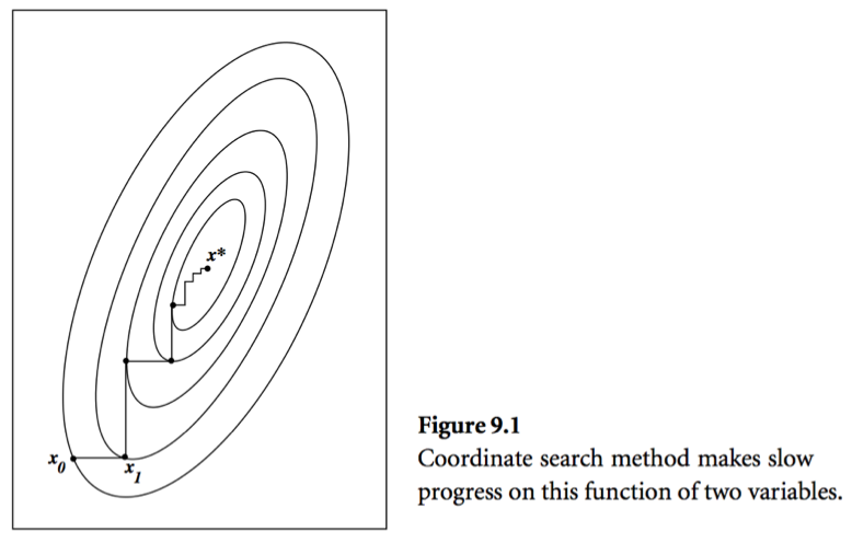
Consider a simple idea: coordinate descent, that is to update $x_j$ alternatingly. Same as the Gauss-Seidel iteration.

A set of vectors $\{\mathbf{x}^{(0)},\ldots,\mathbf{x}^{(l)}\}$ is said to be conjugate with respect to $\mathbf{A}$ if $$ \begin{eqnarray*} \mathbf{p}_i^T \mathbf{A} \mathbf{p}_j = 0, \quad \text{for all } i \ne j. \end{eqnarray*} $$
Conjugate direction method: Given a set of conjugate vectors $\{\mathbf{p}^{(0)},\ldots,\mathbf{p}^{(l)}\}$, at iteration $t$, we search along the conjugate direction $\mathbf{p}^{(t)}$ $$ \begin{eqnarray*} \mathbf{x}^{(t+1)} = \mathbf{x}^{(t)} + \alpha^{(t)} \mathbf{p}^{(t)}, \end{eqnarray*} $$ where $$ \begin{eqnarray*} \alpha^{(t)} = - \frac{\mathbf{r}^{(t)T} \mathbf{p}^{(t)}}{\mathbf{p}^{(t)T} \mathbf{A} \mathbf{p}^{(t)}} \end{eqnarray*} $$ is the optimal step length.
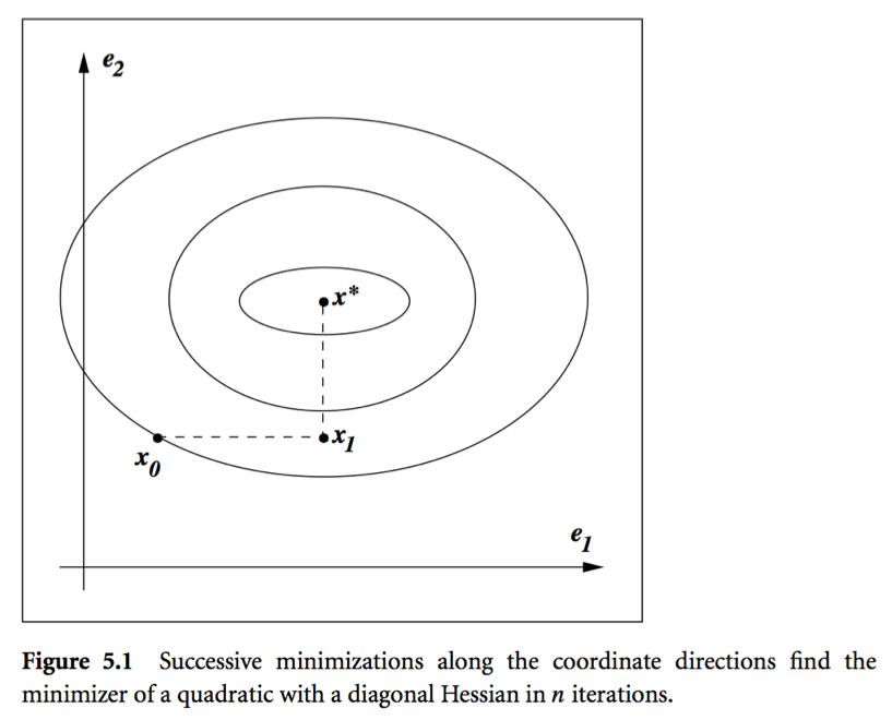
Theorem: In conjugate direction method, $\mathbf{x}^{(t)}$ converges to the solution in at most $n$ steps.

Intuition: Look at graph.

Conjugate gradient method. Idea: generate $\mathbf{p}^{(t)}$ using only $\mathbf{p}^{(t-1)}$ $$ \begin{eqnarray*} \mathbf{p}^{(t)} = - \mathbf{r}^{(t)} + \beta^{(t)} \mathbf{p}^{(t-1)}, \end{eqnarray*} $$ where $\beta^{(t)}$ is determined by the conjugacy condition $\mathbf{p}^{(t-1)T} \mathbf{A} \mathbf{p}^{(t)} = 0$ $$ \begin{eqnarray*} \beta^{(t)} = \frac{\mathbf{r}^{(t)T} \mathbf{A} \mathbf{p}^{(t-1)}}{\mathbf{p}^{(t-1)T} \mathbf{A} \mathbf{p}^{(t-1)}}. \end{eqnarray*} $$
CG algorithm (preliminary version):
1. Given $\mathbf{x}^{(0)}$
2. Initialize: $\mathbf{r}^{(0)} \gets \mathbf{A} \mathbf{x}^{(0)} - \mathbf{b}$, $\mathbf{p}^{(0)} \gets - \mathbf{r}^{(0)}$, $t=0$
3. While $\mathbf{r}^{(0)} \ne \mathbf{0}$
  1. $\alpha^{(t)} \gets - \frac{\mathbf{r}^{(t)T} \mathbf{p}^{(t)}}{\mathbf{p}^{(t)T} \mathbf{A} \mathbf{p}^{(t)}}$
  2. $\mathbf{x}^{(t+1)} \gets \mathbf{x}^{(t)} + \alpha^{(t)} \mathbf{p}^{(t)}$
  3. $\mathbf{r}^{(t+1)} \gets \mathbf{A} \mathbf{x}^{(t+1)} - \mathbf{b}$
  4. $\beta^{(t+1)} \gets \frac{\mathbf{r}^{(t+1)T} \mathbf{A} \mathbf{p}^{(t)}}{\mathbf{p}^{(t)T} \mathbf{A} \mathbf{p}^{(t)}}$
  5. $\mathbf{p}^{(t+1)} \gets - \mathbf{r}^{(t+1)} + \beta^{(t+1)} \mathbf{p}^{(t)}$
  6. $t \gets t+1$
Theorem: With CG algorithm
1. $\mathbf{r}^{(t)}$ are mutually orthogonal.
2. $\{\mathbf{r}^{(0)},\ldots,\mathbf{r}^{(t)}\}$ is contained in the Krylov subspace of degree $t$ for $\mathbf{r}^{(0)}$, denoted by $$ \begin{eqnarray*} {\cal K}(\mathbf{r}^{(0)}; t) = \text{span} \{\mathbf{r}^{(0)},\mathbf{A} \mathbf{r}^{(0)}, \mathbf{A}^2 \mathbf{r}^{(0)}, \ldots, \mathbf{A}^{t} \mathbf{r}^{(0)}\}. \end{eqnarray*} $$
3. $\{\mathbf{p}^{(0)},\ldots,\mathbf{p}^{(t)}\}$ is contained in ${\cal K}(\mathbf{r}^{(0)}; t)$.
4. $\mathbf{p}^{(0)}, \ldots, \mathbf{p}^{(t)}$ are conjugate with respect to $\mathbf{A}$.
  The iterates $\mathbf{x}^{(t)}$ converge to the solution in at most $n$ steps.
CG algorithm (economical version): saves one matrix-vector multiplication.
1. Given $\mathbf{x}^{(0)}$
2. Initialize: $\mathbf{r}^{(0)} \gets \mathbf{A} \mathbf{x}^{(0)} - \mathbf{b}$, $\mathbf{p}^{(0)} \gets - \mathbf{r}^{(0)}$, $t=0$
3. While $\mathbf{r}^{(0)} \ne \mathbf{0}$
  1. $\alpha^{(t)} \gets \frac{\mathbf{r}^{(t)T} \mathbf{r}^{(t)}}{\mathbf{p}^{(t)T} \mathbf{A} \mathbf{p}^{(t)}}$
  2. $\mathbf{x}^{(t+1)} \gets \mathbf{x}^{(t)} + \alpha^{(t)} \mathbf{p}^{(t)}$
  3. $\mathbf{r}^{(t+1)} \gets \mathbf{r}^{(t)} + \alpha^{(t)} \mathbf{A} \mathbf{p}^{(t)}$
  4. $\beta^{(t+1)} \gets \frac{\mathbf{r}^{(t+1)T} \mathbf{r}^{(t+1)}}{\mathbf{r}^{(t)T} \mathbf{r}^{(t)}}$
  5. $\mathbf{p}^{(t+1)} \gets - \mathbf{r}^{(t+1)} + \beta^{(t+1)} \mathbf{p}^{(t)}$
  6. $t \gets t+1$
Computation cost per iteration is one matrix vector multiplication: $\mathbf{A} \mathbf{p}^{(t)}$.
Consider PageRank problem, $\mathbf{A}$ has dimension $n \approx 10^{10}$ but is highly structured (sparse + low rank). Each matrix vector multiplication takes $O(n)$.
Theorem: If $\mathbf{A}$ has $r$ distinct eigenvalues, $\mathbf{x}^{(t)}$ converges to solution $\mathbf{x}^*$ in at most $r$ steps.

Pre-conditioned conjugate gradient (PCG)¶

Summary of conjugate gradient method for solving $\mathbf{A} \mathbf{x} = \mathbf{b}$ or equivalently minimizing $\frac 12 \mathbf{x}^T \mathbf{A} \mathbf{x} - \mathbf{b}^T \mathbf{x}$:
- Each iteration needs one matrix vector multiplication: $\mathbf{A} \mathbf{p}^{(t+1)}$. For structured $\mathbf{A}$, often $O(n)$ cost per iteration.
- Guaranteed to converge in $n$ steps.
Two important bounds for conjugate gradient algorithm:

Let $\lambda_1 \le \cdots \le \lambda_n$ be the ordered eigenvalues of a pd $\mathbf{A}$.
$$ \begin{eqnarray*} \|\mathbf{x}^{(t+1)} - \mathbf{x}^*\|_{\mathbf{A}}^2 &\le& \left( \frac{\lambda_{n-t} - \lambda_1}{\lambda_{n-t} + \lambda_1} \right)^2 \|\mathbf{x}^{(0)} - \mathbf{x}^*\|_{\mathbf{A}}^2 \\ \|\mathbf{x}^{(t+1)} - \mathbf{x}^*\|_{\mathbf{A}}^2 &\le& 2 \left( \frac{\sqrt{\kappa(\mathbf{A})}-1}{\sqrt{\kappa(\mathbf{A})}+1} \right)^{t} \|\mathbf{x}^{(0)} - \mathbf{x}^*\|_{\mathbf{A}}^2, \end{eqnarray*} $$ where $\kappa(\mathbf{A}) = \lambda_n/\lambda_1$ is the condition number of $\mathbf{A}$.

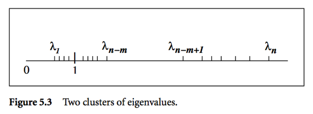
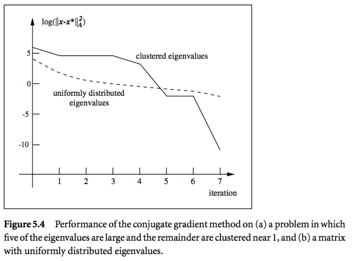
Messages:
- Roughly speaking, if the eigenvalues of $\mathbf{A}$ occur in $r$ distinct clusters, the CG iterates will approximately solve the problem after $O(r)$ steps.
- $\mathbf{A}$ with a small condition number ($\lambda_1 \approx \lambda_n$) converges fast.
Pre-conditioning: Change of variables $\widehat{\mathbf{x}} = \mathbf{C} \mathbf{x}$ via a nonsingular $\mathbf{C}$ and solve $$ (\mathbf{C}^{-T} \mathbf{A} \mathbf{C}^{-1}) \widehat{\mathbf{x}} = \mathbf{C}^{-T} \mathbf{b}. $$ Choose $\mathbf{C}$ such that
- $\mathbf{C}^{-T} \mathbf{A} \mathbf{C}^{-1}$ has small condition number, or
- $\mathbf{C}^{-T} \mathbf{A} \mathbf{C}^{-1}$ has clustered eigenvalues
- Inexpensive solution of $\mathbf{C}^T \mathbf{C} \mathbf{y} = \mathbf{r}$
Preconditioned CG does not make use of $\mathbf{C}$ explicitly, but rather the matrix $\mathbf{M} = \mathbf{C}^T \mathbf{C}$.

Preconditioned CG (PCG) algorithm:
1. Given $\mathbf{x}^{(0)}$, pre-conditioner $\mathbf{M}$
2. $\mathbf{r}^{(0)} \gets \mathbf{A} \mathbf{x}^{(0)} - \mathbf{b}$
3. solve $\mathbf{M} \mathbf{y}^{(0)} = \mathbf{r}^{(0)}$ for $\mathbf{y}^{(0)}$
4. $\mathbf{p}^{(0)} \gets - \mathbf{r}^{(0)}$, $t=0$
5. While $\mathbf{r}^{(0)} \ne \mathbf{0}$
  1. $\alpha^{(t)} \gets \frac{\mathbf{r}^{(t)T} \mathbf{y}^{(t)}}{\mathbf{p}^{(t)T} \mathbf{A} \mathbf{p}^{(t)}}$
  2. $\mathbf{x}^{(t+1)} \gets \mathbf{x}^{(t)} + \alpha^{(t)} \mathbf{p}^{(t)}$
  3. $\mathbf{r}^{(t+1)} \gets \mathbf{r}^{(t)} + \alpha^{(t)} \mathbf{A} \mathbf{p}^{(t)}$
  4. Solve $\mathbf{M} \mathbf{y}^{(t+1)} \gets \mathbf{r}^{(t+1)}$ for $\mathbf{y}^{(t+1)}$
  5. $\beta^{(t+1)} \gets \frac{\mathbf{r}^{(t+1)T} \mathbf{y}^{(t+1)}}{\mathbf{r}^{(t)T} \mathbf{r}^{(t)}}$
  6. $\mathbf{p}^{(t+1)} \gets - \mathbf{y}^{(t+1)} + \beta^{(t+1)} \mathbf{p}^{(t)}$
  7. $t \gets t+1$
  Remark: Only extra cost in the pre-conditioned CG algorithm is the need to solve the linear system $\mathbf{M} \mathbf{y} = \mathbf{r}$.
Pre-conditioning is more like an art than science. Some choices include
- Incomplete Cholesky. $\mathbf{A} \approx \tilde{\mathbf{L}} \tilde{\mathbf{L}}^T$, where $\tilde{\mathbf{L}}$ is a sparse approximate Cholesky factor. Then $\tilde{\mathbf{L}}^{-1} \mathbf{A} \tilde{\mathbf{L}}^{-T} \approx \mathbf{I}$ (perfectly conditioned) and $\mathbf{M} \mathbf{y} = \tilde{\mathbf{L}} \tilde {\mathbf{L}}^T \mathbf{y} = \mathbf{r}$ is easy to solve.
- Banded pre-conditioners.
- Choose $\mathbf{M}$ as a coarsened version of $\mathbf{A}$.
- Subject knowledge. Knowledge about the structure and origin of a problem is often the key to devising efficient pre-conditioner. For example, see recent work of Stein, Chen, Anitescu (2012) for pre-conditioning large covariance matrices. http://epubs.siam.org/doi/abs/10.1137/110834469

Other Krylov subspace methods¶

We leant about CG/PCG, which is for solving $\mathbf{A} \mathbf{x} = \mathbf{b}$, $\mathbf{A}$ pd.
MINRES (minimum residual method): symmetric indefinite $\mathbf{A}$.
Bi-CG (bi-conjugate gradient): unsymmetric $\mathbf{A}$.
Bi-CGSTAB (Bi-CG stabilized): improved version of Bi-CG.
GMRES (generalized minimum residual method): current de facto method for unsymmetric $\mathbf{A}$. E.g., PageRank problem.
Lanczos method: top eigen-pairs of a large symmetric matrix.
Arnoldi method: top eigen-pairs of a large unsymmetric matrix.
Lanczos bidiagonalization algorithm: top singular triplets of large matrix.
LSQR: least square problem $\min \|\mathbf{y} - \mathbf{X} \beta\|_2^2$. Algebraically equivalent to applying CG to the normal equation $(\mathbf{X}^T \mathbf{X} + \lambda^2 I)\mathbf{x} = \mathbf{X}^T \mathbf{y}$.
LSMR: least square problem $\min \|\mathbf{y} - \mathbf{X} \beta\|_2^2$. Algebraically equivalent to applying MINRES to the normal equation $(\mathbf{X}^T \mathbf{X} + \lambda^2 I)\mathbf{x} = \mathbf{X}^T \mathbf{y}$.

Software¶

Matlab¶

Iterative methods for solving linear equations:
pcg, bicg, bicgstab, gmres, ...
Iterative methods for top eigen-pairs and singular pairs:
eigs, svds, ...
Pre-conditioner:
cholinc, luinc, ...
Get familiar with the reverse communication interface (RCI) for utilizing iterative solvers:
```
x = gmres(A, b)
x = gmres(@Afun, b)
eigs(A)}
eigs(@Afun)
```

Julia¶

eigs, svds. Numerical examples
IterativeSolvers.jl package. CG numerical examples
Least squares examples:

using BenchmarkTools, IterativeSolvers

srand(280) # seed
n, p = 1000, 500
X = sprandn(n, p, 0.01)
β = ones(p)
y = X * β + randn(n)

β̂_qr = X \ y
@benchmark X \ y

BenchmarkTools.Trial: 
  memory estimate:  5.17 MiB
  allocs estimate:  99
  --------------
  minimum time:     34.501 ms (0.00% GC)
  median time:      35.069 ms (0.00% GC)
  mean time:        35.273 ms (0.19% GC)
  maximum time:     41.274 ms (0.00% GC)
  --------------
  samples:          142
  evals/sample:     1

β̂_lsqr = lsqr(X, y)
@show vecnorm(β̂_qr - β̂_lsqr)
@benchmark lsqr(X, y)

vecnorm(β̂_qr - β̂_lsqr) = 1.0991691311686633e-5

BenchmarkTools.Trial: 
  memory estimate:  59.03 KiB
  allocs estimate:  463
  --------------
  minimum time:     1.635 ms (0.00% GC)
  median time:      1.663 ms (0.00% GC)
  mean time:        1.773 ms (0.36% GC)
  maximum time:     6.264 ms (71.36% GC)
  --------------
  samples:          2809
  evals/sample:     1

β̂_lsmr = lsqr(X, y)
@show vecnorm(β̂_qr - β̂_lsmr)
@benchmark lsmr(X, y)

vecnorm(β̂_qr - β̂_lsmr) = 1.0991691311686633e-5

BenchmarkTools.Trial: 
  memory estimate:  34.33 KiB
  allocs estimate:  272
  --------------
  minimum time:     1.030 ms (0.00% GC)
  median time:      1.044 ms (0.00% GC)
  mean time:        1.113 ms (0.39% GC)
  maximum time:     5.332 ms (73.24% GC)
  --------------
  samples:          4469
  evals/sample:     1